Sine and Cosine Function Graphs - AP Precalculus

SECTION 1

Historical Context & Motivation

The study of sine and cosine functions stretches back thousands of years, rooted in the practical needs of astronomy and land surveying. Ancient civilizations recognized that circular motion generates predictable, repeating patterns—patterns that could be captured numerically and used to predict celestial events with remarkable accuracy. The transition from tabular values to continuous wave-shaped graphs was a conceptual leap that unified geometry, algebra, and analysis, ultimately providing the mathematical language for describing periodic phenomena throughout the sciences.

~150 CE • Ptolemy's Chord Tables

Claudius Ptolemy compiled a table of chords in his Almagest, effectively tabulating values equivalent to the sine function for use in astronomical calculations.

~500 CE • Indian Half-Chord (Jyā)

Indian mathematician Aryabhata introduced the jyā (half-chord), the direct ancestor of the modern sine function, along with its complement, the kojyā, corresponding to cosine.

1635 • Roberval's Sinusoidal Curve

Gilles de Roberval became one of the first mathematicians to sketch the sine function as a continuous curve on a Cartesian-style coordinate system, revealing its wave-like shape.

1748 • Euler's Analytic Formulation

Leonhard Euler, in Introductio in analysin infinitorum, defined sine and cosine as functions of a real variable using the unit circle, establishing the modern framework for their graphical analysis.

1822 • Fourier's Harmonic Analysis

Joseph Fourier demonstrated that virtually any periodic function can be decomposed into a sum of sine and cosine waves, making these graphs foundational to physics and engineering.

This historical arc reveals a central question: how can we precisely describe, transform, and interpret the characteristic wave-shaped graphs produced by sine and cosine? The AP Precalculus course requires you to fluently read these graphs, connect their features to algebraic parameters, and apply transformations—skills that rest on understanding the underlying unit-circle definitions and the geometric meaning of each parameter.

SECTION 2

Core Principles & Definitions

Before graphing sine and cosine, you must internalize a small set of foundational ideas that govern the behavior of every sinusoidal curve. Each principle connects an algebraic parameter to a visual feature of the graph, creating a two-way fluency: given an equation, you can sketch the graph, and given a graph, you can write the equation. The following grid distills these principles.

Unit-Circle Origin

For any angle θ on the unit circle, the coordinates of the terminal point are (cos θ, sin θ). Plotting the y-coordinate against θ yields the sine graph; plotting the x-coordinate yields the cosine graph.

Periodicity

Both sine and cosine complete one full cycle every 2π radians. The period T = 2π/|B| when a frequency factor B is applied: f(x) = sin(Bx). A larger |B| compresses the wave horizontally.

Amplitude

The amplitude |A| measures the maximum vertical displacement from the midline. In y = A sin(x), the graph oscillates between A and −A (assuming no vertical shift).

Phase Shift & Vertical Shift

A phase shift C/B translates the graph horizontally, while a vertical shift D raises or lowers the midline. Together these position the wave anywhere in the coordinate plane.

Sine–Cosine Relationship

Cosine is a phase-shifted sine: cos(x) = sin(x + π/2). Graphically, the cosine curve is the sine curve shifted π/2 units to the left, so every property of one function transfers directly to the other.

✦

KEY TAKEAWAY

Think of a sinusoidal graph as a circular motion "unrolled" onto a flat timeline. Imagine a point traveling counterclockwise around the unit circle while a strip of paper scrolls past, recording the point's height at each instant. The amplitude is the circle's radius, the period is the time for one full revolution, the phase shift is where on the circle you start, and the vertical shift is how high you mount the circle above the ground. Every transformation to the equation simply changes one of those physical settings.

SECTION 3

Visual Explanation — Parent Sine & Cosine Graphs

The solid cyan curve is y = sin(x) and the dashed violet curve is y = cos(x). Note that cosine leads sine by π/2 radians: every feature of the cosine graph appears π/2 units earlier on the x-axis. The amber annotation marks the amplitude, and the green bracket marks one full period of 2π.

Several features are immediately visible. The sine function begins at the origin (0, 0), rises to its maximum of 1 at x = π/2, returns to 0 at x = π, reaches its minimum of −1 at x = 3π/2, and completes the cycle back at 0 when x = 2π. The cosine function follows the identical shape but starts at its maximum: (0, 1). Both curves are smooth, continuous, and unbounded in domain—they extend infinitely in both directions along the x-axis while their range remains locked to [−1, 1]. Recognizing these key points—intercepts, maxima, and minima—at quarter-period intervals is the single most efficient strategy for sketching either graph by hand.

💡

AP Exam Tip

Free-response questions frequently ask you to identify the five key points of one cycle (start, first quarter, midpoint, third quarter, end). Practice plotting these for both sin and cos so you can sketch quickly under time pressure.

SECTION 4

Mathematical Framework — The General Sinusoidal Model

The parent functions y = sin(x) and y = cos(x) are special cases of a more powerful general form. By introducing four parameters—amplitude, frequency, phase shift, and vertical shift—we can model any sinusoidal behavior. The AP Precalculus course expects fluency in moving between the equation and the graph in both directions.

GENERAL SINUSOIDAL FORM

y = A sin(B(x − C)) + D or y = A cos(B(x − C)) + D

A = amplitude (|A| is the distance from midline to peak; if A < 0, the graph reflects over the midline). B = frequency factor (period T = 2π / |B|). C = phase (horizontal) shift (positive C shifts right). D = vertical shift (midline is y = D).

PERIOD

T = 2π / |B|

The period is the horizontal length of one complete cycle. Doubling B halves the period, compressing the wave horizontally.

RANGE

[D − |A|, D + |A|]

The output values oscillate symmetrically about the midline y = D. The maximum value is D + |A| and the minimum is D − |A|.

SINE–COSINE PHASE IDENTITY

cos(x) = sin(x + π/2) and sin(x) = cos(x − π/2)

This identity confirms that cosine and sine are the same wave separated by a quarter-period phase shift. Any sinusoidal function can be written equivalently in either form by adjusting C.

A critical subtlety involves the sign conventions. When the equation is written as y = A sin(B(x − C)) + D, the phase shift is +C (rightward). However, some textbooks factor differently: y = A sin(Bx − φ) + D, in which case the phase shift is φ/B. On the AP exam, carefully identify which form is being used before extracting the shift. Always verify your reading by checking whether the key points of the graph match your algebraic predictions.

⚠

Common Pitfall

Students frequently confuse the sign of the phase shift. Remember: in y = sin(B(x − C)), replacing x with (x − C) shifts the graph to the right by C units. If you see y = sin(2x + π), first factor: y = sin(2(x + π/2)), so the phase shift is −π/2, meaning the graph shifts π/2 to the left.

SECTION 5

Detailed Breakdown — Transformations of Sinusoidal Graphs

Understanding how each parameter transforms the parent graph is essential for the AP Precalculus exam. Rather than memorizing isolated rules, it is more productive to see each transformation as a geometric operation applied to the parent curve's five key points. The diagram below illustrates how amplitude, period, phase shift, and vertical shift independently alter the graph of y = sin(x).

Four panels showing individual transformations applied to the parent sine curve (dashed gray). Top-left (pink): amplitude doubled. Top-right (amber): period halved to π. Bottom-left (cyan): phase shift right by π/2. Bottom-right (emerald): vertical shift up by 1, midline now at y = 1.

Transformation	Parameter Changed	Effect on Graph	Effect on Key Points
Vertical Stretch/Compression	\|A\| ≠ 1	Stretches (\|A\| > 1) or compresses (0 < \|A\| < 1) vertically	Multiply all y-values by A
Reflection over midline	A < 0	Maxima become minima and vice versa	Negate y-displacements from midline
Horizontal Stretch/Compression	\|B\| ≠ 1	Period changes to 2π/\|B\|	Divide all x-values by B
Phase Shift	C ≠ 0	Entire graph translates horizontally	Add C to all x-values
Vertical Shift	D ≠ 0	Midline moves to y = D	Add D to all y-values

Summary of sinusoidal transformations and their effects

SECTION 6

Worked Example — Graphing a Transformed Sinusoid

Let us graph the function y = −3 cos(2(x − π/4)) + 1 and identify all key features. This example combines every transformation: amplitude change, reflection, period change, phase shift, and vertical shift.

Graph y = −3 cos(2(x − π/4)) + 1

1
Step 1 — Identify Parameters

Compare y = −3 cos(2(x − π/4)) + 1 to the general form y = A cos(B(x − C)) + D. We read off: A = −3, B = 2, C = π/4, D = 1.

A = −3, B = 2, C = π/4, D = 1
2
Step 2 — Determine Amplitude and Reflection

The amplitude is |A| = |−3| = 3. Because A is negative, the graph is reflected over its midline: the parent cosine starts at a maximum, but this graph starts at a minimum.

Amplitude = 3, reflected (starts at minimum)
3
Step 3 — Compute the Period

Period T = 2π / |B| = 2π / 2 = π. One full cycle now spans π radians, half the parent cosine's period.

Period = π
4
Step 4 — Identify Phase Shift and Vertical Shift

The phase shift is C = π/4 to the right. The vertical shift is D = 1, so the midline is y = 1 instead of y = 0. The range is [D − |A|, D + |A|] = [1 − 3, 1 + 3] = [−2, 4].

Phase shift = π/4 right; midline y = 1; range [−2, 4]
5
Step 5 — Plot the Five Key Points

For y = cos(x), the five key points over one cycle [0, 2π] are: (0, 1), (π/2, 0), (π, −1), (3π/2, 0), (2π, 1). Apply transformations in order: divide x by B, add C, multiply y by A, add D. Original → After B: divide x by 2 → After C: add π/4 → After A and D: y becomes −3y + 1. (0, 1) → (0, 1) → (π/4, 1) → (π/4, −3(1)+1) = (π/4, −2) (π/2, 0) → (π/4, 0) → (π/2, 0) → (π/2, −3(0)+1) = (π/2, 1) (π, −1) → (π/2, −1) → (3π/4, −1) → (3π/4, −3(−1)+1) = (3π/4, 4) (3π/2, 0) → (3π/4, 0) → (π, 0) → (π, −3(0)+1) = (π, 1) (2π, 1) → (π, 1) → (5π/4, 1) → (5π/4, −3(1)+1) = (5π/4, −2)

Key points: (π/4, −2), (π/2, 1), (3π/4, 4), (π, 1), (5π/4, −2)
6
Step 6 — Sketch and Verify

Plot the five key points, draw a smooth sinusoidal curve through them, and verify: the minimum is −2 (occurring at x = π/4 and 5π/4), the maximum is 4 (at x = 3π/4), the midline crossings occur at x = π/2 and x = π, and the horizontal distance from minimum to minimum is π, confirming the period.

Graph complete. One cycle spans [π/4, 5π/4], midline y = 1, amplitude 3, reflected cosine.

SECTION 7

Comparing Sine and Cosine — Strengths & Modeling Choices

Because sine and cosine differ only by a phase shift, any sinusoidal model can be written using either function. However, choosing wisely can simplify both the equation and its interpretation. The table below highlights practical considerations for modeling and exam contexts.

Feature	y = A sin(B(x − C)) + D	y = A cos(B(x − C)) + D
Starting behavior (at x = C)	Starts at midline, moving upward (A > 0)	Starts at maximum (A > 0)
Symmetry	Odd function: sin(−x) = −sin(x)	Even function: cos(−x) = cos(x)
Best used when data...	Starts at the midline value (e.g., spring at equilibrium)	Starts at an extreme value (e.g., height at top of Ferris wheel)
Derivative relationship	d/dx [sin(x)] = cos(x)	d/dx [cos(x)] = −sin(x)
Conversion	sin(x) = cos(x − π/2)	cos(x) = sin(x + π/2)

Practical comparison of sine and cosine forms for modeling

🔑

MODELING INSIGHT

Think of choosing between sine and cosine like choosing between measuring longitude from Greenwich or from the International Date Line—you're describing the same globe, just anchored to different starting references. Pick the form that makes the phase shift C equal to zero (or as simple as possible) given the data's starting behavior. This reduces algebraic complexity and minimizes sign errors.

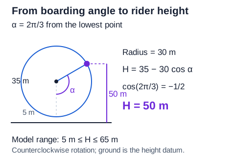A Ferris wheel accompanies a circular height diagram with radius 30 m, center 35 m above ground and a bottom starting position; a 2π/3 turn reaches 50 m. Suppose a wheel has radius 30 m and center height 35 m. Starting at the bottom gives H(α) = 35 − 30 cos α: amplitude 30 m, midline 35 m, and range 5–65 m.

SECTION 8

Connections to Advanced Theory

The graphical analysis of sine and cosine is not an endpoint but a gateway. In calculus, the smooth oscillating behavior of these functions yields elegant derivative and integral relationships. In physics and engineering, the sinusoidal model underpins wave mechanics, alternating-current circuits, and signal processing. Even within the AP Precalculus course itself, the graphical concepts extend to other trigonometric functions and to polar curves.

Concept in This Lesson	Advanced Extension	Where It Appears
Amplitude and period	Fourier series: any periodic function = sum of sinusoids with specific amplitudes and periods	AP Physics, multivariable calculus, signal processing
Phase shift	Phasor representation of AC circuits; complex exponential form $e^{iθ}$ = cos θ + i sin θ	AP Physics C, electrical engineering
Sinusoidal shape (concavity)	Second derivative test: d²/dx² sin(x) = −sin(x), showing inflection points coincide with zeros	AP Calculus AB/BC
Graphing y = sin(x) on Cartesian plane	Graphing r = sin(θ) on the polar plane produces a circle; r = a + b sin(θ) yields limaçons and cardioids	AP Precalculus Unit 3 (Polar)
Range [D − \|A\|, D + \|A\|]	Bounded output → the squeeze theorem for limits involving sin(x)/x and oscillating products	AP Calculus AB/BC limits unit

How sine and cosine graph concepts extend into advanced mathematics and science

Mastering the graphical behavior of sine and cosine now gives you a transferable skill set. When you encounter damped oscillations (y = $e^{−kx}$ sin(x)) in differential equations, or when you analyze resonance in physics, you will rely on the same five-key-point strategy, the same parameter-reading techniques, and the same transformation logic developed in this lesson. The language of sinusoids is one of the most widely spoken in all of STEM.

SECTION 9

Practice Problems

Question 1: CONCEPTUAL

Which of the following correctly describes the relationship between the graphs of y = sin(x) and y = cos(x)?

A. The graph of y = cos(x) is a reflection of y = sin(x) over the x-axis.
B. The graph of y = cos(x) is the graph of y = sin(x) shifted π/2 units to the left.
C. The graph of y = cos(x) is the graph of y = sin(x) shifted π units to the right.
D. The graph of y = cos(x) is a vertical stretch of y = sin(x) by a factor of 2.
E. The graph of y = cos(x) is the graph of y = sin(x) shifted π/2 units to the right.

Show answer (B)

B is correct. The identity cos(x) = sin(x + π/2) shows that the cosine graph is obtained by shifting the sine graph π/2 units to the left. Choice A is wrong because reflection over the x-axis would produce y = −sin(x), which is not cosine. Choice C is incorrect because a shift of π would give sin(x − π) = −sin(x), not cos(x). Choice D is wrong because sine and cosine have the same amplitude; no vertical scaling is involved. Choice E describes a rightward shift, which would give sin(x − π/2) = −cos(x), introducing a reflection as well.

Question 2: BASIC CALCULATION

What is the period of the function y = 4 sin(3x) − 2?

A. 3π
B. 2π/3
C. 6π
D. π/3
E. 2π

Show answer (B)

B is correct. Using the period formula T = 2π/|B| with B = 3, we get T = 2π/3. Choice A (3π) incorrectly multiplies 3 by π instead of dividing 2π by 3. Choice C (6π) incorrectly multiplies 2π by 3. Choice D (π/3) divides π rather than 2π by 3. Choice E (2π) is the period of the parent function and ignores the frequency factor entirely. The amplitude (4) and vertical shift (−2) do not affect the period.

Question 3: INTERMEDIATE

A sinusoidal function has a maximum value of 7, a minimum value of 1, and completes one full cycle over the interval [0, 4π]. If the function reaches its maximum at x = π, which of the following is a correct equation?

A. y = 3 cos(x/2 − π/2) + 4
B. y = 6 cos(x/2 − π) + 1
C. y = 3 sin(2x − π) + 4
D. y = 3 cos(x − π) + 4
E. y = 3 cos(x/2) + 4

Show answer (A)

A is correct. The amplitude is (7 − 1)/2 = 3 and the midline is (7 + 1)/2 = 4, so D = 4 and |A| = 3. The period is 4π, giving |B| = 2π/(4π) = 1/2. Since the maximum occurs at x = π, using cosine form: y = 3 cos((1/2)(x − π)) + 4 = 3 cos(x/2 − π/2) + 4. Checking: at x = π, cos(π/2 − π/2) = cos(0) = 1, so y = 3(1) + 4 = 7 ✓. Choice B has amplitude 6, which is too large. Choice C uses B = 2, giving period π, not 4π. Choice D uses B = 1, giving period 2π, not 4π. Choice E has no phase shift, so the maximum would be at x = 0, not x = π.

Question 4: APPLIED

4 pts

The water depth at a coastal dock varies sinusoidally with time due to tidal forces. At 2:00 AM, the water depth reaches its maximum of 14 feet. At 8:00 AM, the depth reaches its minimum of 6 feet. (a) Find the amplitude, period, midline, and phase shift for a cosine model of the form D(t) = A cos(B(t − C)) + D, where t is measured in hours after midnight. (b) Write the complete equation for D(t). (c) Determine the water depth at 5:00 AM. (d) A boat requires at least 11 feet of water to safely dock. During one full tidal cycle starting at 2:00 AM, determine the total number of hours when the boat can safely dock.

Show answer

Rubric (4 points): Point 1 — Parameters (Part a): Amplitude = (14 − 6)/2 = 4 ft. Midline = (14 + 6)/2 = 10 ft (D = 10). The time from maximum (2 AM) to minimum (8 AM) is 6 hours, which is half a period, so the full period = 12 hours. B = 2π/12 = π/6. Since the maximum occurs at t = 2, the phase shift C = 2. Point 2 — Equation (Part b): D(t) = 4 cos(π/6 (t − 2)) + 10. Point 3 — Evaluation (Part c): At t = 5: D(5) = 4 cos(π/6 (5 − 2)) + 10 = 4 cos(π/2) + 10 = 4(0) + 10 = 10 feet. Point 4 — Inequality (Part d): Solve D(t) ≥ 11: 4 cos(π/6 (t − 2)) + 10 ≥ 11 → cos(π/6 (t − 2)) ≥ 1/4. Let u = π/6(t − 2). We need cos(u) ≥ 1/4. Within one period [0, 2π], cos(u) ≥ 1/4 when u ∈ [0, arccos(1/4)] ∪ [2π − arccos(1/4), 2π]. arccos(1/4) ≈ 1.318 radians. The total u-length where cos(u) ≥ 1/4 is 2 × arccos(1/4) ≈ 2.636 radians. Converting to hours: Δt = 2.636/(π/6) = 2.636 × 6/π ≈ 5.03 hours. The boat can safely dock for approximately 5 hours per tidal cycle.

Question 5: CRITICAL THINKING

3 pts

A student claims that the function f(x) = 2 sin(x) + 3 cos(x) is not sinusoidal because it is a sum of two different trigonometric functions. Refute this claim by: (a) Expressing f(x) in the form R sin(x + φ), where R > 0 and 0 ≤ φ < 2π. (b) Stating the amplitude, period, and phase shift of f(x). (c) Explaining in one or two sentences why any linear combination a sin(x) + b cos(x) must be sinusoidal.

Show answer

Rubric (3 points): Point 1 — Conversion (Part a): We use the identity a sin(x) + b cos(x) = R sin(x + φ), where R = √(a² + b²) and tan(φ) = b/a. Here a = 2, b = 3, so R = √(4 + 9) = √13. tan(φ) = 3/2, so φ = arctan(3/2) ≈ 0.983 radians. Since both a and b are positive, φ is in the first quadrant. Thus f(x) = √13 sin(x + arctan(3/2)). Point 2 — Features (Part b): Amplitude = √13 ≈ 3.606. Period = 2π (since B = 1). Phase shift = arctan(3/2) ≈ 0.983 radians to the left. Point 3 — Justification (Part c): Any linear combination a sin(x) + b cos(x) can be rewritten as a single sinusoidal function R sin(x + φ) using the sine addition formula, because the sum formula sin(x + φ) = sin(x)cos(φ) + cos(x)sin(φ) shows that any such combination is simply one sinusoid with amplitude R = √(a² + b²) and an appropriate phase angle. The sum of two sinusoids of the same frequency is always a sinusoid of that same frequency.

SUMMARY

Lesson Summary

Summary

The graphs of sine and cosine are smooth, continuous, periodic waves that originate from the unit circle. The parent functions oscillate between −1 and 1 with a period of 2π and an amplitude of 1. The general sinusoidal model y = A sin(B(x − C)) + D (or its cosine equivalent) encodes four transformations: amplitude |A| stretches or compresses vertically, frequency B sets the period to 2π/|B|, phase shift C translates horizontally, and vertical shift D raises or lowers the midline.

The key graphing strategy is to identify the five key points (start, quarter, midpoint, three-quarter, end) of one cycle, apply transformations to each point, and connect them with a smooth curve. Cosine is simply sine shifted by π/2 to the left, so every technique for one function transfers directly to the other. Mastery of these graphs is essential not only for the AP Precalculus exam but also as the foundation for Fourier analysis, polar curves, and calculus-based wave mechanics.