Semi-log Plots - AP Precalculus

SECTION 1

Historical Context & Motivation

When scientists first began collecting data on phenomena such as bacterial growth, radioactive decay, and compound interest, they quickly noticed a recurring problem: the numbers grew (or shrank) so rapidly that plotting them on ordinary graph paper produced curves that were either cramped near zero or rocketed off the page. A semi-log plot was the elegant solution—by applying a logarithmic scale to one axis, the explosive curvature of exponential data collapses into a manageable straight line, making trends visible and parameters easy to extract.

1614 • Napier Publishes Logarithms

John Napier's Mirifici Logarithmorum Canonis Descriptio introduced logarithms as a computational tool, laying the algebraic groundwork that would later enable logarithmic scaling.

1780s • Logarithmic Graph Scales Emerge

Engineers and surveyors began experimenting with unevenly spaced rulings on graph paper to linearize exponential relationships in cartography and physics.

1846 • Commercial Log-Scale Paper

Printed semi-logarithmic graph paper became commercially available, allowing scientists to plot data directly and read off exponential rates from the slope of a line.

20th c. • Standard Tool in Sciences

Semi-log plots became indispensable in fields ranging from electronics (Bode plots) to biology (growth curves) and finance (long-run stock charts).

The central question this lesson addresses is deceptively simple: How can we tell whether a data set is truly exponential, and how do we extract its base and initial value? The semi-log plot answers both questions at once—if the transformed data forms a line, the relationship is exponential, and the slope and intercept encode the parameters of the model.

SECTION 2

Core Principles & Definitions

A semi-log plot is a graph in which one axis (typically the vertical axis) uses a logarithmic scale while the other axis retains a standard linear scale. The power of this arrangement rests on a single algebraic identity: taking the logarithm of an exponential function yields a linear function. Understanding the following foundational ideas will equip you to read, construct, and interpret semi-log plots on the AP Precalculus exam.

Logarithmic Axis

Instead of equal spacing between tick marks, each decade (factor of 10) occupies the same physical distance. The axis effectively plots log(y) in place of y.

Linearization

If y =

ab^x

, then log(y) = log(a) + x·log(b). This is the equation of a line in the variables x and log(y), with slope log(b) and y-intercept log(a).

Linearity Test

Data that forms a straight line on a semi-log plot is exponential. Curvature on the semi-log plot means the original data is not purely exponential.

Slope ↔ Growth/Decay Rate

A positive slope indicates exponential growth; a negative slope indicates exponential decay. A steeper line means a larger base b (faster change).

✦

KEY TAKEAWAY

Think of a semi-log plot as a translator. Exponential data speaks a 'curved' language on regular axes; the logarithmic scale acts like a decoder ring that converts that curve into a straight line you already know how to analyze with slope and intercept.

SECTION 3

Visual Explanation

The diagram below places two plots side by side. On the left, the exponential function y = 2(3)^x is graphed on standard linear axes—notice how the curve accelerates steeply upward. On the right, the same data is plotted on a semi-log grid where the vertical axis is scaled by log₁₀; the result is a straight line whose slope equals log(3) ≈ 0.477.

Left: y = 2·3^x on linear axes shows the characteristic exponential curve. Right: the same data on a semi-log plot produces a straight line with slope log(3) ≈ 0.477 and vertical intercept log(2) ≈ 0.301.

Notice how the five data points on the left panel (x = 0, 1, 2, 3, 4 corresponding to y = 2, 6, 18, 54, 162) hug the x-axis for small values and then surge upward—this makes it difficult to read any intermediate values with precision. On the semi-log plot in the right panel, the same points fall neatly on a line because the vertical axis is scaled by log₁₀. The constant spacing between consecutive points along the vertical direction confirms that the ratio between successive y-values is constant—the hallmark of an exponential function.

SECTION 4

Mathematical Framework

The algebraic justification for semi-log plots hinges on the logarithmic transformation of an exponential model. Suppose a quantity y depends on x according to the general exponential form. Applying the common logarithm (log₁₀) to both sides converts the equation into a linear form whose parameters are directly readable from the graph.

EXPONENTIAL MODEL

y = a · b^x (a > 0, b > 0, b ≠ 1)

a = initial value (y-value when x = 0), b = base (constant multiplicative factor per unit increase in x).

LOGARITHMIC TRANSFORMATION

log₁₀(y) = log₁₀(a) + x · log₁₀(b)

Letting Y = log₁₀(y), this becomes Y = log₁₀(a) + log₁₀(b) · x, a linear equation in x and Y.

SLOPE AND INTERCEPT

slope m = log₁₀(b) ⟹ b = 10^m ; Y-intercept = log₁₀(a) ⟹ a = 10^(Y-intercept)

The slope of the line on the semi-log plot encodes the base b, and the vertical intercept encodes the initial value a. Recover both by exponentiating with base 10.

ℹ

Natural Log Variant

If the vertical axis uses ln (log base e) instead of log₁₀, the slope equals ln(b) and the intercept equals ln(a). The AP exam typically uses log₁₀, but the principle is identical for any logarithm base.

This framework reveals why semi-log plots are so powerful for data analysis. Determining whether a data set is exponential reduces to a visual linearity check, and extracting the model parameters requires only computing the slope and intercept of the best-fit line, then raising 10 to those values.

SECTION 5

Reading & Constructing Semi-log Plots

On the AP Precalculus exam, you may be given a semi-log plot and asked to determine the exponential model, or given data and asked to decide which type of plot linearizes it. The diagram below illustrates how to read key features: the y-intercept of the line gives log₁₀(a), two well-separated points let you compute the slope, and the sign of the slope tells you whether the model describes growth or decay.

The green dashed segment marks the y-intercept log₁₀(a) ≈ 0.4, giving a = 10^0.4 ≈ 2.512. The pink rise-over-run triangle shows a slope of 0.4, so b = 10^0.4 ≈ 2.512 as well.

Step 1 — Identify two points on the line. Choose points far apart for accuracy, such as (x₁, log y₁) and (x₂, log y₂).
Step 2 — Compute slope. m = (log y₂ − log y₁) / (x₂ − x₁). This equals log₁₀(b).
Step 3 — Recover b. b = $10^m$ .
Step 4 — Recover a. a = $10^{Y-intercept}$ , where the Y-intercept is log₁₀(y) at x = 0.

SECTION 6

Worked Example

A biologist measures the number of bacteria in a culture at regular one-hour intervals. She plots the data on a semi-log graph (log₁₀ of population vs. time in hours) and observes a straight line passing through the points (0, 2) and (5, 3.5). Determine the exponential model for the population P as a function of time t.

Finding the Exponential Model from a Semi-log Line

1
Step 1 — Identify the linear form

On the semi-log plot the vertical coordinate is log₁₀(P) and the horizontal coordinate is t. The equation of the line is log₁₀(P) = mt + c, where m is the slope and c is the vertical intercept.
2
Step 2 — Calculate the slope

Using the two given points (t₁, log P₁) = (0, 2) and (t₂, log P₂) = (5, 3.5): m = (3.5 − 2) / (5 − 0) = 1.5 / 5 = 0.3.

m = 0.3
3
Step 3 — Read the intercept

At t = 0 the semi-log plot gives log₁₀(P) = 2, so c = 2.

c = 2
4
Step 4 — Recover b and a

The base is b = $10^m$ = $10^{0.3}$ ≈ 1.995 ≈ 2, and the initial value is a = $10^c$ = 10² = 100.

b ≈ 2, a = 100
5
Step 5 — Write the model

The exponential model is P(t) = 100 · $2^t$ . The population doubles every hour, starting from 100 bacteria.

P(t) = 100 · $2^t$

A researcher looks through a microscope beside a closed culture vessel,sample containers and an illustrative cell inset. The line log₁₀P = 0.3t + 2 gives P = 100×10^(0.3t). Its hourly growth factor is about 1.995.

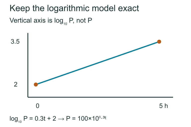The line log₁₀P = 0.3t + 2 gives P = 100×10^(0.3t). Its hourly growth factor is about 1.995.

SECTION 7

Semi-log vs. Linear and Log-log Plots

Semi-log plots are one member of a family of transformed-axis plots. Choosing the right plot type depends on the suspected relationship between variables. The table below compares three common options so you can quickly decide which is appropriate for a given data set—an important skill tested in the free-response section of the AP Precalculus exam.

Feature	Linear Plot	Semi-log Plot	Log-log Plot
Axes	Both linear	x linear, y logarithmic	Both logarithmic
Linearizes	y = mx + c (linear)	y = a· $b^x$ (exponential)	y = a· $x^n$ (power)
Slope gives	Rate of change m	log₁₀(b)	Exponent n
Intercept gives	y-intercept c	log₁₀(a)	log₁₀(a)
Typical use	Constant-rate processes	Population growth, radioactive decay, compound interest	Allometric scaling, Kepler's law

Comparison of three common plot types used to linearize data

✦

KEY TAKEAWAY

If you see a straight line on a semi-log plot, the data is exponential—the same way seeing a straight line on a regular plot tells you the data is linear. If the line on a semi-log plot curves, try a log-log plot; a straight line there means you have a power function instead.

SECTION 8

Connection to Regression & Advanced Theory

On the AP Precalculus exam, the semi-log plot serves as a graphical gateway to exponential regression. In a statistics or calculus course, you would use least-squares regression on the transformed data (x, log y) to find the best-fit line, then convert the parameters back to the exponential scale. The table below connects the semi-log concepts you have learned to their more advanced counterparts.

AP Precalculus Concept	Advanced Extension
Visual linearity check on semi-log plot	Residual analysis and R² value in exponential regression
Slope = log₁₀(b)	Continuous growth rate k when model is y = $ae^{kx}$ , slope = k/ln(10)
Common log (base 10)	Natural log (base e) preferred in calculus for differentiation
Two-point slope calculation	Least-squares fit minimizing Σ(log yᵢ − (mx + c))²

The semi-log framework also connects to the broader idea of function transformations that pervade AP Precalculus and beyond. Whenever a relationship appears nonlinear, applying the right transformation—logarithmic, reciprocal, square root—can reveal hidden linearity and make the underlying model accessible through the simple tools of slope-intercept analysis.

SECTION 9

Practice Problems

Question 1: CONCEPTUAL

A set of data is plotted on a semi-log graph (log₁₀(y) on the vertical axis, x on the horizontal axis) and the points form a straight line. Which of the following best describes the original relationship between x and y?

A. y = mx + c (linear)
B. y = ax² (quadratic)
C. y = a · $b^x$ (exponential)
D. y = a · ln(x) (logarithmic)
E. y = a/x (reciprocal)

Show answer (C)

The correct answer is (C). A straight line on a semi-log plot means log₁₀(y) = mx + c, which exponentiates to y =

10^c

(10^m)^x

= a ·

b^x

, an exponential function. (A) y = mx + c is linear and would appear as a line on a standard plot, not necessarily on a semi-log plot. (B) y = ax² is a power/quadratic function, which would linearize on a log-log plot, not a semi-log plot. (D) y = a · ln(x) is a logarithmic function, which does not produce a line on semi-log axes. (E) y = a/x is a reciprocal function, which would not linearize on a semi-log plot.

Question 2: BASIC CALCULATION

On a semi-log plot, a line passes through (1, 1.2) and (4, 2.1), where the vertical axis represents log₁₀(y). What is the value of the base b in the exponential model y = a ·

b^x

A. b ≈ 1.68
B. b ≈ 2.00
C. b ≈ 7.94
D. b = 0.3
E. b ≈ 2.82

Show answer (B)

The correct answer is (B). The slope of the semi-log line is m = (2.1 − 1.2)/(4 − 1) = 0.9/3 = 0.3, so b =

10^{0.3}

≈ 2.0. (A)

10^{0.225}

≈ 1.68, which would result from dividing 0.9 by 4 instead of 3. (C)

10^{0.9}

≈ 7.94, which mistakes the numerator of the slope (Δ log y) for the slope itself. (D) 0.3 confuses the slope m = log₁₀(b) with b itself. (E)

10^{0.45}

≈ 2.82, which would result from dividing 0.9 by 2.

Question 3: INTERMEDIATE

A semi-log plot of data produces a line with y-intercept 3 and slope −0.2 (where the vertical axis is log₁₀(y) and the horizontal axis is x). Which of the following is the corresponding exponential model?

A. y = 1000 $(0.2)^x$
B. y = 3 $(0.631)^x$
C. y = 1000 $(1.585)^x$
D. y = 1000 $(0.631)^x$
E. y = 0.631 $(1000)^x$

Show answer (D)

The correct answer is (D). From the semi-log line log₁₀(y) = −0.2x + 3, we get a = 10³ = 1000 and b =

10^{−0.2}

≈ 0.631, so y = 1000

(0.631)^x

. The negative slope indicates exponential decay (b < 1). (A) is wrong because it uses b = 0.2 rather than

10^{−0.2}

. (B) uses a = 3 instead of 10³. (C) has the correct a but uses b =

10^{0.2}

≈ 1.585 (growth instead of decay). (E) reverses the roles of a and b.

Question 4: APPLIED

4 pts

A pharmacologist measures the concentration C (in mg/L) of a drug in a patient's bloodstream at various times t (in hours) after injection. When log₁₀(C) is plotted against t, the data fall on a line passing through (0, 1.7) and (6, 0.5). (a) Write the exponential model C(t). (b) Determine the drug's half-life (the time for the concentration to halve). (c) Predict the concentration at t = 10 hours.

Show answer

(a) [2 points] Slope m = (0.5 − 1.7)/(6 − 0) = −1.2/6 = −0.2. Intercept c = 1.7, so a =

10^{1.7}

≈ 50.12 mg/L and b =

10^{−0.2}

≈ 0.6310. Model: C(t) = 50.12 ·

(0.6310)^t

. (b) [1 point] Half-life: 50.12 ·

(0.6310)^t

₁/₂ = 25.06 ⟹

(0.6310)^t

₁/₂ = 0.5 ⟹ t₁/₂ = log(0.5)/log(0.6310) = (−0.3010)/(−0.2) = 1.505 hours ≈ 1.5 hours. (c) [1 point] C(10) = 50.12 ·

(0.6310)^{10}

= 50.12 ·

10^{−2}

= 50.12 · 0.01 = 0.5012 mg/L ≈ 0.50 mg/L.

Question 5: CRITICAL THINKING

3 pts

A student plots experimental data on a semi-log graph and observes that the points are close to a straight line but with a slight upward curve for large x-values. (a) Explain what this curvature suggests about the data's departure from a purely exponential model. (b) Propose a different type of transformed plot the student could try and explain why. (c) If the student insists on using an exponential model for only the linear portion (small x-values), describe how the slope of that segment relates to the short-term growth rate.

Show answer

(a) [1 point] The upward curvature on the semi-log plot means that for large x, the data grows faster than any single exponential a·

b^x

can predict. This could indicate a power-function component, a second exponential term with a larger base, or a transition to super-exponential growth. (b) [1 point] The student could try a log-log plot (both axes logarithmic). If the data straightens there, the underlying model is a power function y =

ax^n

rather than exponential. Alternatively, plotting log(y) versus x² could reveal Gaussian-type growth. (c) [1 point] The slope of the linear segment on the semi-log plot for small x equals log₁₀(b), where b is the short-term multiplicative growth factor per unit x. The short-term growth rate per unit x is b − 1 (expressed as a decimal), and the model y = a·

b^x

would be valid only over the range of x where the semi-log data is approximately linear.

SUMMARY

Lesson Summary

Summary

A semi-log plot graphs data with a logarithmic vertical axis and a linear horizontal axis. When data of the form y = a · b^x is plotted this way, the result is a straight line because the logarithmic transformation converts the exponential relationship into the linear form log₁₀(y) = log₁₀(a) + x · log₁₀(b).

The slope of the semi-log line equals log₁₀(b), so the base is recovered as b = 10^slope. The y-intercept equals log₁₀(a), giving a = 10^intercept. A positive slope signals exponential growth (b > 1), while a negative slope signals exponential decay (0 < b < 1). If the data curves on the semi-log plot, the relationship is not purely exponential—consider a log-log plot to test for a power model instead.