Polar Function Graphs - AP Precalculus

SECTION 1

Historical Context & Motivation

Long before the familiar x-y grid became the default language of analytic geometry, mathematicians recognized that certain curves — spirals, petals, and closed loops — resist clean description in rectangular coordinates. The polar coordinate system arose precisely to address this limitation, offering a framework in which distance from an origin and angle from a reference direction serve as the two fundamental measurements. This system transforms complicated algebraic expressions into strikingly simple equations, revealing underlying symmetry that Cartesian representations obscure.

~200 BCE • Archimedean Spiral

Archimedes of Syracuse studied the spiral that now bears his name — a curve traced by a point moving outward from the origin at constant speed while rotating at constant angular velocity — laying informal groundwork for radius-angle thinking.

1637 • Cartesian Coordinates Formalized

René Descartes published La Géométrie, establishing the rectangular coordinate system. While transformative, it highlighted the clumsiness of expressing curves like cardioids and limaçons in x-y form.

1691 • Jakob Bernoulli & the Lemniscate

Jakob Bernoulli investigated the figure-eight lemniscate, a curve whose polar equation r² = a² cos 2θ is far simpler than its Cartesian equivalent, demonstrating the descriptive power of polar representation.

1748 • Euler's Introductio

Leonhard Euler systematized the polar coordinate system in Introductio in analysin infinitorum, formalizing the notation (r, θ) and establishing conventions for graphing polar functions that remain standard today.

Modern • AP Precalculus Curriculum

Polar functions appear in the AP Precalculus framework as a bridge between trigonometric reasoning and the calculus of parametric and polar curves, preparing students for integration in polar coordinates.

The central question that motivates this lesson is deceptively simple: given a rule r = f(θ), how do we visualize the resulting curve in the plane, determine its symmetry, and identify its key features? Answering this question requires understanding how the interplay of radius and angle generates shapes that are both beautiful and analytically powerful — from the spiral paths of galaxies to the radiation patterns of antennas.

SECTION 2

Core Principles & Definitions

Before graphing any polar function, you need a firm grasp of the coordinate system itself and the conventions that govern how curves are traced. In polar coordinates, every point in the plane is specified by an ordered pair (r, θ), where r is the directed distance from the pole (origin) and θ is the angle measured counterclockwise from the polar axis (positive x-axis). A critical distinction from Cartesian coordinates is that negative values of r are meaningful: when r < 0, the point is plotted in the direction opposite to angle θ.

The Pole & Polar Axis

The pole is the fixed origin, and the polar axis is the initial ray (typically horizontal, pointing right). All angles θ are measured from this reference direction, with positive angles counterclockwise.

Directed Radius r

The value r represents a signed distance. When r > 0, the point lies along the ray at angle θ; when r < 0, the point lies along the ray at angle θ + π. This convention allows a single equation to trace curves that cross through the pole.

Non-Unique Representation

Unlike Cartesian coordinates, every polar point has infinitely many names. For example, (2, π/3), (2, π/3 + 2π), and (−2, π/3 + π) all describe the same location. This non-uniqueness affects symmetry testing.

Conversion Formulas

To bridge polar and Cartesian systems: x = r cos θ, y = r sin θ, r² = x² + y², and tan θ = y/x. These conversions are essential for verifying graphs and simplifying certain polar equations.

Symmetry Tests

Replace θ with −θ to test for polar-axis symmetry, replace θ with π − θ for symmetry about θ = π/2, and replace r with −r for symmetry about the pole. If any substitution yields an equivalent equation, the corresponding symmetry is confirmed.

✦

KEY TAKEAWAY

Think of polar graphing like a radar sweep: the angle θ is the direction the beam points, and r is the distance a blip appears from the center of the screen. As the beam rotates through all angles, every blip r = f(θ) traces out the curve — just as radar paints the outline of a coastline one angular slice at a time.

SECTION 3

Visual Explanation — The Polar Grid

A polar grid consists of concentric circles (constant r) and radial rays (constant θ). The cyan curve shows the cardioid r = 3 + 3 cos θ. Notice how the curve passes through the pole when r = 0 at θ = π and achieves its maximum r = 6 at θ = 0.

The diagram above illustrates the essential structure of polar graphing. Concentric circles mark constant values of r, while radial lines emanate at standard angles — 0, π/6, π/4, π/3, π/2, and their multiples. When graphing a polar function r = f(θ), you evaluate f at each angle, measure the resulting distance outward along that ray, and then connect the plotted points smoothly. The cardioid shown is a member of the limaçon family of curves — specifically, the special case where the loop just touches the pole without crossing through it. This characteristic heart shape emerges whenever the equation takes the form r = a + a cos θ or r = a + a sin θ, making the coefficients equal.

💡

AP Exam Tip

On the AP Precalculus exam, you may be asked to identify features of a polar graph — such as where the curve passes through the pole, the number of petals, or the maximum value of r — without a calculator. Practice building a quick θ-r value table at key angles (0, π/6, π/4, π/3, π/2, etc.) to sketch curves by hand.

SECTION 4

Mathematical Framework

The algebraic machinery behind polar graphs involves several families of equations, each producing a characteristic shape. Understanding these canonical forms allows you to predict the shape of a polar curve before plotting a single point. The following equations and their properties form the backbone of the AP Precalculus polar graphing toolkit.

CIRCLES THROUGH THE POLE

r = a cos θ or r = a sin θ

These equations produce circles of diameter |a|. The cosine version is centered on the polar axis (x-axis); the sine version is centered on the line θ = π/2 (y-axis). The parameter a determines the diameter, with the circle passing through the pole.

ROSE CURVES

r = a cos(nθ) or r = a sin(nθ)

Rose curves produce petal-shaped patterns. When n is odd, the rose has exactly n petals; when n is even, the rose has 2n petals. Each petal extends to a maximum distance of |a| from the pole. The angle between consecutive petals is π/n for an odd n and π/(2n) for an even n.

LIMAÇONS

r = a ± b cos θ or r = a ± b sin θ

The ratio a/b determines the limaçon's shape: if a/b < 1, there is an inner loop; if a/b = 1, the curve is a cardioid; if 1 < a/b < 2, a dimpled limaçon appears; if a/b ≥ 2, the curve is convex (no dimple). The parameter a shifts the curve away from the pole, while b controls the amplitude of oscillation.

LEMNISCATES

r² = a² cos 2θ or r² = a² sin 2θ

Lemniscates are figure-eight curves symmetric about the pole. The cosine version is symmetric about both the polar axis and the line θ = π/2; the sine version is symmetric about the lines θ = π/4 and θ = 3π/4. Only angles where cos 2θ ≥ 0 (or sin 2θ ≥ 0) produce real values of r.

When Does r = 0? Identifying Pole Passages

A polar curve passes through the pole whenever f(θ) = 0 for some value of θ. These angles are critical because they mark the directions along which the curve arrives at and departs from the origin. For example, the rose r = 4 sin 3θ equals zero when 3θ = 0, π, 2π, 3π, … , i.e., θ = 0, π/3, 2π/3, π. Each of these angles represents a boundary between petals, and plotting them first establishes the angular framework of the curve.

Maximum and Minimum Values of r

The maximum value of |r| determines how far the curve extends from the pole, and the angles at which this maximum occurs identify the tips of petals, the outermost point of a limaçon, or the widest part of a circle. For r = a + b cos θ, the maximum value of r is |a| + |b| occurring at θ = 0 (for the "+" case), and the minimum value is |a| − |b|. If this minimum is negative, the curve has an inner loop. For rose curves r = a cos(nθ), the maximum distance is simply |a|, occurring at angles where cos(nθ) = ±1.

SECTION 5

Detailed Breakdown of Polar Curve Families

Polar curves can be organized into distinct families based on their equations and the shapes they produce. The diagram below compares four fundamental curve types side by side, illustrating how different equations yield dramatically different geometries. Mastering these families is essential for the AP exam, where you will be expected to match equations to graphs and analyze features without extensive computation.

Four fundamental families of polar curves: the cardioid (a special limaçon), the rose curve, the lemniscate, and the circle through the pole. The reference box below summarizes the petal-counting rule for rose curves.

Curve Family	General Equation	Key Feature	Passes Through Pole?
Circle	r = a cos θ or r = a sin θ	Diameter = \|a\|, centered at (a/2, 0) or (0, a/2)	Yes
Cardioid	r = a ± a cos θ or r = a ± a sin θ	Heart-shaped; a/b = 1	Yes (once)
Limaçon with loop	r = a + b cos θ (a/b < 1)	Inner loop when \|a\| < \|b\|	Yes (twice)
Rose	r = a cos(nθ) or r = a sin(nθ)	n odd → n petals; n even → 2n petals	Yes (between petals)
Lemniscate	r² = a² cos 2θ or r² = a² sin 2θ	Figure-eight; symmetric about the pole	Yes (center crossing)

Summary of the five most-tested polar curve families on the AP Precalculus exam.

SECTION 6

Worked Example — Graphing a Rose Curve

Let us graph the polar function r = 4 sin 2θ completely, identifying all key features. This is a rose curve with n = 2, so we expect 2n = 4 petals.

Graphing r = 4 sin 2θ

1
Step 1 — Identify the Curve Type

The equation has the form r = a sin(nθ) with a = 4 and n = 2. Since n = 2 is even, the rose curve will have 2n = 4 petals. Each petal extends a maximum distance of |a| = 4 from the pole.

4-petal rose, maximum r = 4
2
Step 2 — Find Where r = 0 (Pole Passages)

Set 4 sin 2θ = 0, so sin 2θ = 0, giving 2θ = 0, π, 2π, 3π, 4π. Therefore θ = 0, π/2, π, 3π/2, 2π. These five angles (four distinct directions in [0, 2π)) mark the boundaries between petals.

r = 0 at θ = 0, π/2, π, 3π/2
3
Step 3 — Find Maximum r (Petal Tips)

The maximum of |sin 2θ| is 1, occurring when 2θ = π/2, 3π/2, 5π/2, 7π/2, i.e., θ = π/4, 3π/4, 5π/4, 7π/4. At θ = π/4 and 5π/4, sin 2θ = 1 so r = 4 (positive, plotted along the ray). At θ = 3π/4 and 7π/4, sin 2θ = −1 so r = −4 (plotted opposite the ray direction). Each of these four angles corresponds to the tip of a petal.

Petal tips at θ = π/4, 3π/4, 5π/4, 7π/4 with |r| = 4
4
Step 4 — Build a Value Table

Evaluate r at several key angles: θ = 0 → r = 0; θ = π/6 → r = 4 sin(π/3) = 4(√3/2) = 2√3 ≈ 3.46; θ = π/4 → r = 4 sin(π/2) = 4; θ = π/3 → r = 4 sin(2π/3) = 4(√3/2) = 2√3 ≈ 3.46; θ = π/2 → r = 4 sin π = 0. This traces one complete petal from θ = 0 to θ = π/2. The pattern repeats for the remaining three quadrants.

Each petal spans a π/2 interval of θ
5
Step 5 — Check Symmetry

Replace θ with −θ: r = 4 sin(−2θ) = −4 sin 2θ ≠ 4 sin 2θ, so the curve is not symmetric about the polar axis by this test alone. However, replacing r with −r and θ with −θ: −r = −4 sin 2θ gives r = 4 sin 2θ ✓, confirming symmetry about the pole. Additionally, replacing θ with π − θ: r = 4 sin(2π − 2θ) = −4 sin 2θ, and since replacing r with −r restores the original equation, the curve also has symmetry about θ = π/2. Together, these confirm the four-fold symmetry we expect.

Symmetric about the pole and θ = π/2
6
Step 6 — Sketch the Graph

Plot the points from the value table on polar graph paper, connecting them smoothly. The first petal rises from the pole along θ = 0, reaches its tip at (4, π/4) in the first quadrant, and returns to the pole at θ = π/2. The remaining three petals appear in quadrants II, III, and IV, each oriented at π/4, 3π/4, 5π/4, and 7π/4 respectively, creating a four-petal flower centered at the origin.

Four petals in quadrants I–IV, tips on the lines θ = π/4, 3π/4, 5π/4, 7π/4

SECTION 7

Polar vs. Cartesian — Strengths & Limitations

Neither polar nor Cartesian coordinates are universally superior — each system has domains where it excels and situations where it introduces unnecessary complexity. Understanding when to use polar representation versus rectangular representation is itself a testable skill on the AP exam and a valuable mathematical habit of mind.

Feature	Polar Coordinates	Cartesian Coordinates
Curves with rotational symmetry	Natural fit — circles, roses, spirals have simple equations	Often requires implicit or parametric forms; equations are complicated
Linear functions	Cumbersome; a line through the origin is θ = c, but other lines require r = a / (b cos θ + c sin θ)	Simple: y = mx + b
Point representation	Non-unique — infinitely many (r, θ) pairs for each point	Unique — exactly one (x, y) pair per point
Intersection finding	Tricky — must also check the pole separately due to non-unique representations	Straightforward — set equations equal and solve
Applications	Antenna patterns, orbital mechanics, microphone pickup patterns, fluid flow around cylinders	Architecture, engineering blueprints, standard data plotting, linear models

When to choose polar vs. Cartesian representation.

✦

KEY TAKEAWAY

Choosing between polar and Cartesian coordinates is like choosing between a wrench and a screwdriver — neither is inherently better, but using the right tool for the job can reduce a complicated problem to a single clean equation. Whenever a curve exhibits radial symmetry or is most naturally described by distance and direction from a center point, polar coordinates will almost certainly yield a simpler representation.

SECTION 8

Connection to Advanced Theory

The polar graphing skills you develop in AP Precalculus form the foundation for several important topics in calculus and beyond. In AP Calculus BC, you will compute areas enclosed by polar curves using the integral A = (1/2)∫r² dθ, and you will find arc lengths using ds = √(r² + (dr/dθ)²) dθ. The ability to identify where a curve passes through the pole, where it reaches maximum r, and which intervals of θ trace distinct portions of the curve directly determines how you set up these integrals.

AP Precalculus Skill	Advanced Extension
Plotting r = f(θ) and identifying key features	Setting up bounds for polar area integrals in Calculus BC
Analyzing maximum and minimum values of r	Finding extreme distances and tangent lines using dr/dθ
Recognizing rose, limaçon, and lemniscate families	Complex analysis (z = $re^{iθ}$ ), Fourier analysis of periodic patterns
Converting between polar and Cartesian forms	Multivariable calculus: polar double integrals, Jacobian determinant
Symmetry analysis of polar curves	Group theory applications in physics and crystallography

How AP Precalculus polar skills connect to advanced mathematics.

Beyond pure mathematics, polar functions model real phenomena with remarkable elegance. The radiation pattern of a dipole antenna is a figure-eight described by r = cos θ, while cardioid microphones derive their name from the heart-shaped polar sensitivity pattern r = 1 + cos θ. In orbital mechanics, Kepler's first law states that planetary orbits are ellipses with the Sun at one focus — an ellipse whose polar equation r = a(1 − e²)/(1 + e cos θ) directly encodes the eccentricity e and semi-major axis a.

SECTION 9

Practice Problems

Question 1: CONCEPTUAL

The polar curve r = 5 cos 3θ is a rose curve. How many petals does it have, and what is the maximum distance from the pole to the curve?

A. 3 petals, maximum distance 5
B. 6 petals, maximum distance 5
C. 3 petals, maximum distance 15
D. 6 petals, maximum distance 15
E. 3 petals, maximum distance 3

Show answer (A)

For a rose curve r = a cos(nθ), when n is odd, the number of petals equals n, and when n is even, the number equals 2n. Here n = 3 (odd), so the curve has exactly 3 petals. The maximum value of |r| equals |a| = 5, occurring when cos 3θ = ±1. Choice B is incorrect because the 2n rule applies only when n is even. Choice C incorrectly multiplies a × n for the maximum distance. Choice D makes both the even-n petal error and the multiplication error. Choice E incorrectly uses n instead of a for the maximum distance.

Question 2: BASIC CALCULATION

At which angle θ in the interval [0, 2π) does the polar curve r = 2 + 4 sin θ pass through the pole?

A. θ = π/6
B. θ = 7π/6 and θ = 11π/6
C. θ = π/2
D. θ = 3π/2
E. The curve never passes through the pole

Show answer (B)

Setting r = 0 gives 2 + 4 sin θ = 0, so sin θ = −1/2. In [0, 2π), sin θ = −1/2 at θ = 7π/6 and θ = 11π/6. Choice A is incorrect because sin(π/6) = 1/2, which would give r = 4 rather than 0. Choice C gives r = 2 + 4(1) = 6, the maximum value. Choice D gives r = 2 + 4(−1) = −2, which is nonzero (the point is plotted in the opposite direction, not at the pole). Choice E is incorrect because a/b = 2/4 = 1/2 < 1, so this limaçon has an inner loop that necessarily passes through the pole.

Question 3: INTERMEDIATE

Which of the following polar equations produces a limaçon with an inner loop?

A. r = 5 + 3 cos θ
B. r = 4 + 4 sin θ
C. r = 2 + 5 cos θ
D. r = 6 + 3 sin θ
E. r = 3 cos 2θ

Show answer (C)

For a limaçon r = a + b cos θ or r = a + b sin θ, an inner loop occurs when |a/b| < 1, meaning |a| < |b|. In choice C, a = 2 and b = 5, so a/b = 2/5 < 1, producing an inner loop. Choice A has a/b = 5/3 > 1, giving a convex limaçon (no dimple, since a/b ≥ 2 is needed for the convex designation — here 5/3 is between 1 and 2, so it is actually dimpled). Choice B has a/b = 4/4 = 1, which produces a cardioid (no inner loop). Choice D has a/b = 6/3 = 2, yielding a convex limaçon. Choice E is a rose curve, not a limaçon.

Question 4: APPLIED

4 pts

A microphone has a polar sensitivity pattern modeled by r = 3 + 3 cos θ, where r represents the pickup sensitivity (in arbitrary units) at angle θ from the front of the microphone. (a) Identify the type of polar curve and justify your answer. (b) Determine the maximum sensitivity and the angle at which it occurs. (c) Find all angles θ in [0, 2π) where the sensitivity is zero. Explain what this means physically. (d) A sound source is located at angle θ = 2π/3 from the front of the microphone. Calculate the sensitivity at this angle and express it as a fraction of the maximum sensitivity.

Show answer

Point-by-point rubric: (a) [1 point] The equation r = 3 + 3 cos θ has the form r = a + a cos θ with a = 3. Since a/b = 3/3 = 1, this is a cardioid. The equal coefficients confirm that the curve is a cardioid rather than a general limaçon. (b) [1 point] Maximum sensitivity occurs when cos θ = 1, i.e., θ = 0. At θ = 0, r = 3 + 3(1) = 6. The maximum sensitivity is 6 units, occurring directly in front of the microphone. (c) [1 point] Set r = 0: 3 + 3 cos θ = 0 → cos θ = −1 → θ = π. The sensitivity is zero at θ = π, which corresponds to directly behind the microphone. Physically, the microphone rejects all sound arriving from the rear, which is the defining characteristic of a cardioid pickup pattern. (d) [1 point] At θ = 2π/3: r = 3 + 3 cos(2π/3) = 3 + 3(−1/2) = 3 − 3/2 = 3/2. As a fraction of maximum: (3/2)/6 = 1/4. The microphone picks up only one-quarter of its maximum sensitivity at this off-axis angle. Right-facing cardioid sensitivity with front response 6, side response 3 and rear null zero, in arbitrary response units.

Right-facing cardioid sensitivity with front response 6, side response 3 and rear null zero, in arbitrary response units.

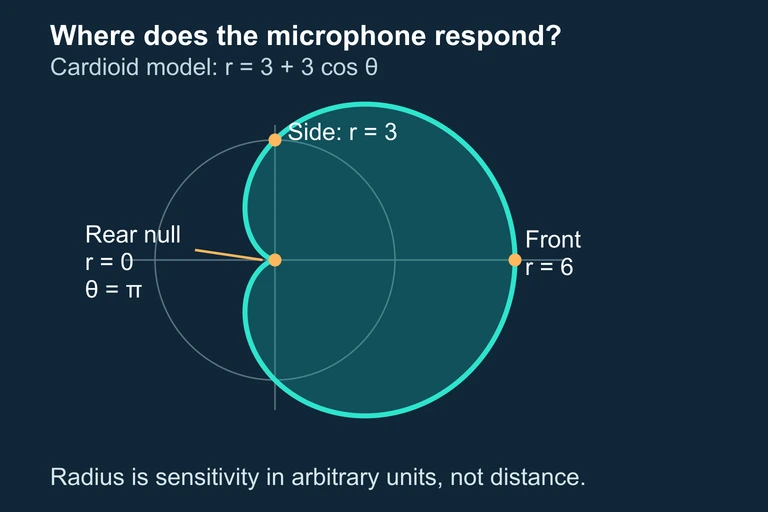The microphone cardioid compares front, side and rear sensitivity; its radial coordinate is not geographic coverage.

Question 5: CRITICAL THINKING

3 pts

Consider the two polar curves r₁ = 2 sin θ and r₂ = 2 cos θ. (a) Convert each equation to Cartesian form to identify the curves geometrically. (b) Find all points of intersection, including any intersection at the pole that may not appear by solving r₁ = r₂ algebraically. (c) Explain why setting r₁ = r₂ does not reveal the intersection at the pole, connecting your explanation to the non-uniqueness of polar representations.

Show answer

Point-by-point rubric: (a) [1 point] Multiply both sides of r₁ = 2 sin θ by r: r² = 2r sin θ → x² + y² = 2y → x² + (y − 1)² = 1. This is a circle centered at (0, 1) with radius 1. Similarly, r₂ = 2 cos θ gives r² = 2r cos θ → x² + y² = 2x → (x − 1)² + y² = 1. This is a circle centered at (1, 0) with radius 1. (b) [1 point] Setting 2 sin θ = 2 cos θ gives tan θ = 1, so θ = π/4 (in [0, π)). At θ = π/4, r = 2 sin(π/4) = √2. In Cartesian form, this point is (1, 1). Both circles also pass through the pole: r₁ = 0 when θ = 0, and r₂ = 0 when θ = π/2. So the pole (0, 0) is the second intersection point. The two intersection points are (1, 1) and (0, 0). (c) [1 point] Setting r₁ = r₂ algebraically requires both functions to equal the same r-value at the same θ-value simultaneously. The pole is represented as (0, 0) for r₁ at θ = 0 and as (0, π/2) for r₂ — these are the same geometric point but with different θ-values. Because the pole has infinitely many polar representations, two curves can intersect there at different parameter values, making the intersection invisible to the algebraic method. This is why one must always check the pole separately.

SUMMARY

Lesson Summary

Summary

Polar function graphs describe curves using the relationship r = f(θ), where each point is determined by a directed distance r from the pole and an angle θ from the polar axis. The major curve families include circles (r = a cos θ or a sin θ), limaçons and cardioids (r = a ± b cos θ, classified by the ratio a/b), rose curves (r = a cos nθ, with n petals if n is odd and 2n petals if n is even), and lemniscates (r² = a² cos 2θ).

To graph any polar function, identify the curve family from its equation, find where r = 0 (pole passages), determine the maximum value of |r| and the angles where it occurs, test for symmetry (about the polar axis, the line θ = π/2, or the pole), and build a θ-r value table at key angles. Remember that polar representations are non-unique, so intersection problems and symmetry tests require careful attention to alternate forms. These skills lay the groundwork for polar area and arc length integrals in Calculus BC and beyond.