

SECTION 1
Historical Context & Motivation
Humans have observed periodic phenomena—events that repeat at regular intervals—since the earliest civilizations tracked the rising and setting of the sun, the phases of the moon, and the cycling of the seasons. These observations were not merely practical; they were the first intuitive encounters with the idea that certain quantities return to the same value after a fixed interval of time or space. The mathematical formalization of periodicity, however, required centuries of intellectual development, stretching from ancient Greek astronomy through the Enlightenment's invention of trigonometric analysis.
~150 CE • Ptolemy's Almagest
1635 • Harmonic Vibrations
1748 • Euler's Formula
1822 • Fourier's Theorem
Modern Era • Digital Signal Processing
The central question that unites all of these developments is deceptively simple: How do we build precise mathematical models for quantities that cycle through the same values over and over again? In AP Precalculus, we answer this question primarily through sinusoidal functions—the sine and cosine families—while also recognizing that periodicity is a broader property shared by tangent, cotangent, and other functions. Mastering this topic means learning to identify, parameterize, and interpret the repeating behavior that governs phenomena from Ferris wheel heights to tidal cycles.
SECTION 2
Core Principles & Definitions
Before diving into equations, it is essential to establish the precise vocabulary that AP Precalculus uses to describe periodic behavior. A function f is called periodic if there exists a positive constant p such that f(x + p) = f(x) for every x in the domain. The smallest such positive value of p is called the period of the function. This definition captures the essence of repetition: after one full period, the function's output values cycle identically. The following grid introduces the five foundational ideas you must command for the AP exam.
Period
Amplitude
Midline
Phase Shift
Frequency
KEY TAKEAWAY
SECTION 3
Visual Explanation — Anatomy of a Sinusoidal Wave
The diagram above captures the four essential parameters that transform the parent functions y = sin x and y = cos x into general sinusoidal models. Notice that the wave oscillates symmetrically about the midline: the maximum value equals D + A and the minimum value equals D − A. The distance between consecutive maxima (or consecutive minima, or any two corresponding points one cycle apart) is exactly the period. On the AP exam, you will frequently be given a graph or a real-world data table and asked to extract these parameters—so train your eye to identify the midline first, then measure the amplitude above it, then count the horizontal distance for one full cycle to determine the period.
SECTION 4
Mathematical Framework
The general sinusoidal model encapsulates all periodic behavior that can be described by sine or cosine. Both forms are equivalent up to a phase shift, since cos x = sin(x + π/2). In AP Precalculus, you should be fluent with both the sine and cosine versions, and you should be able to convert between them.
GENERAL SINE FORM
A = amplitude (|A|, always positive in interpretation; a negative A reflects the wave over the midline). B = frequency parameter (period = 2π/|B|). C = phase shift (horizontal translation). D = vertical shift (midline y = D).
GENERAL COSINE FORM
Same parameters as the sine form. Cosine starts at its maximum when A > 0 and C = 0, whereas sine starts at the midline. Choose whichever form makes the phase shift simpler for the given context.
PERIOD FORMULA
Solving for B when the period T is known: B = 2π / T. For applications measured in time (hours, days), this lets you convert a real-world cycle length directly into the frequency parameter of your model.
AMPLITUDE AND MIDLINE FROM DATA
When given a data set or graph, identify the greatest output value (max) and the least output value (min). These two formulas immediately yield the amplitude and midline without any curve fitting.
AP Exam Tip
SECTION 5
Transformations & Their Graphical Effects
Understanding how each parameter in the general sinusoidal equation transforms the graph is essential for both multiple-choice reasoning and free-response construction. The table below catalogs every transformation, its algebraic effect, and its graphical manifestation. Internalizing this table will allow you to move fluidly between equations, graphs, and verbal descriptions—a skill tested repeatedly on the AP Precalculus exam.
| Parameter Change | Algebraic Effect | Graphical Effect |
|---|---|---|
| Increase |A| | Multiplies all output displacements from midline | Vertical stretch — peaks move farther from midline |
| A < 0 | Negates the sine/cosine output | Reflection over the midline |
| Increase |B| | Period = 2π/|B| decreases | Horizontal compression — more cycles per interval |
| Decrease |B| | Period = 2π/|B| increases | Horizontal stretch — fewer cycles per interval |
| C > 0 | Replaces x with (x − C) | Shift right by C units |
| D ≠ 0 | Adds D to every output | Shifts entire wave up (D > 0) or down (D < 0) |
Summary of how each parameter in f(x) = A sin(B(x − C)) + D affects the graph.
Observe how the violet curve has the same period as the parent but reaches twice as high and twice as low, while the amber curve completes two full cycles in the same horizontal span where the parent completes one. The amber curve's midline sits at y = 1 rather than y = 0, shifting the entire oscillation upward. On the AP exam, questions may present you with one of these transformed graphs and ask you to determine the equation, or vice versa—give you an equation and ask you to identify key features of the graph.
SECTION 6
Worked Example — Modeling Tidal Heights
A coastal town records water levels at a fixed location. On a particular day, the high tide reaches 11.2 feet at 3:00 AM and the low tide drops to 2.8 feet at 9:15 AM. Assuming the water level follows a sinusoidal model as a function of time (in hours after midnight), construct a cosine function that models the height h(t) of the water.
Tidal Height Model
- 1
Step 1 — Find the Midline (D)
The midline is the average of the maximum and minimum heights: D = (max + min) / 2 = (11.2 + 2.8) / 2.D = 7.0 feet - 2
Step 2 — Find the Amplitude (A)
The amplitude is half the distance between the maximum and minimum: A = (max − min) / 2 = (11.2 − 2.8) / 2.A = 4.2 feet - 3
Step 3 — Find the Period and B
The time from high tide to the next low tide is half a period. High tide occurs at t = 3 hours and low tide at t = 9.25 hours (9 hours 15 minutes). So half the period is 9.25 − 3 = 6.25 hours, giving a full period of T = 12.5 hours. Then B = 2π / T = 2π / 12.5.B = 4π/25 ≈ 0.5027 - 4
Step 4 — Find the Phase Shift (C)
We choose the cosine form because cosine reaches its maximum at the start of its cycle. Since the maximum occurs at t = 3, we set C = 3 so that when t = 3 the argument is zero and cos(0) = 1, placing the peak at the correct time.C = 3 - 5
Step 5 — Assemble the Model
Substituting all parameters into the general cosine form h(t) = A cos(B(t − C)) + D yields the final sinusoidal model.h(t) = 4.2 cos((4π/25)(t − 3)) + 7 - 6
Step 6 — Verify
Check: h(3) = 4.2 cos(0) + 7 = 4.2(1) + 7 = 11.2 ✓. h(9.25) = 4.2 cos((4π/25)(6.25)) + 7 = 4.2 cos(π) + 7 = 4.2(−1) + 7 = 2.8 ✓. Both the high and low tide values match the given data.Model verified ✓
 Tide height ranges from 2.8 to 11.2 ft, giving midline 7 ft and amplitude 4.2 ft. The 6.25-hour high-to-low interval is half the 12.5-hour period.
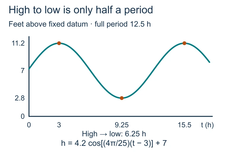 Tide height ranges from 2.8 to 11.2 ft, giving midline 7 ft and amplitude 4.2 ft. The 6.25-hour high-to-low interval is half the 12.5-hour period.
SECTION 7
Sine vs. Cosine — Choosing the Right Form
A common source of confusion for students is when to use the sine form versus the cosine form. Mathematically, the two are interchangeable: any sine function can be rewritten as a cosine with a different phase shift, since sin x = cos(x − π/2). The choice is ultimately about convenience and minimizing the complexity of the phase shift constant. The following table provides a strategic comparison.
| Criterion | Use Sine When… | Use Cosine When… |
|---|---|---|
| Starting point of data | Data begins at the midline and increases | Data begins at the maximum (or minimum if A < 0) |
| Phase shift simplicity | Midline crossing is aligned with a convenient x-value | The peak is aligned with a convenient x-value |
| Convention in context | Often used in physics (e.g., simple harmonic motion from equilibrium) | Often used in tidal, temperature, and engineering models where the peak is the natural starting event |
| Symmetry considerations | Sine is odd: sin(−x) = −sin x, useful when origin symmetry matters | Cosine is even: cos(−x) = cos x, useful when y-axis symmetry matters |
Strategic guide for choosing between sine and cosine forms on the AP Precalculus exam.
KEY TAKEAWAY
SECTION 8
Connections to Advanced Theory
While AP Precalculus focuses primarily on sinusoidal models, periodicity extends far beyond sine and cosine. The tangent function, for instance, is periodic with period π rather than 2π, and it possesses vertical asymptotes that sinusoidal functions lack. Understanding how the sinusoidal framework connects to these more complex periodic functions—and to calculus-level concepts—provides critical context for what lies ahead in your mathematical journey.
| Feature | AP Precalculus (This Course) | AP Calculus & Beyond |
|---|---|---|
| Primary functions | sin, cos, tan and their inverses | All six trig functions, hyperbolic functions, Fourier series |
| Key skill | Constructing sinusoidal models from data or descriptions | Differentiating and integrating periodic functions; Taylor series |
| Decomposition | Model a single periodic behavior with one sinusoid | Fourier analysis: decompose any periodic function into infinite sums of sinusoids |
| Applications | Tides, temperatures, Ferris wheels, daylight hours | Signal processing, quantum mechanics, heat equation, electrical engineering |
| Rate of change | Described qualitatively (increasing/decreasing over intervals) | Computed precisely: d/dx [sin x] = cos x, d/dx [cos x] = −sin x |
How periodicity concepts in AP Precalculus connect to calculus and higher mathematics.
One of the most profound results you will encounter later is that the derivative of a sinusoidal function is itself sinusoidal—sin differentiates to cos, and cos differentiates to −sin. This means the rate of change of a periodic process is also periodic, a fact with deep implications in physics (velocity and acceleration in circular motion) and engineering (alternating current circuits). For now, building strong fluency with the shape, parameters, and behavior of sinusoidal graphs gives you the essential foundation for all of these advanced applications.
SECTION 9
Practice Problems
Question 1: CONCEPTUAL
- A. f(5)
- B. f(8)
- C. f(10)
- D. f(19)
- E. f(24)
Show answer (D)
Question 2: BASIC CALCULATION
- A. Amplitude = 14, Midline y = 3
- B. Amplitude = 7, Midline y = 3
- C. Amplitude = 7, Midline y = 7
- D. Amplitude = 5, Midline y = 3
- E. Amplitude = 7, Midline y = 0
Show answer (B)
Question 3: INTERMEDIATE
- A. t = 0 hours (midnight)
- B. t = 3 hours (3:00 AM)
- C. t = 6 hours (6:00 AM)
- D. t = 12 hours (noon)
- E. t = 9 hours (9:00 AM)
Show answer (A)
Question 4: APPLIED
4 ptsShow answer
Question 5: CRITICAL THINKING
3 ptsShow answer
SUMMARY
Summary — Periodic Phenomena
Summary
A periodic function satisfies f(x + p) = f(x) for all x, where the smallest such positive p is the period. The general sinusoidal model f(x) = A sin(B(x − C)) + D (or its cosine equivalent) is fully determined by four parameters: the amplitude A = (max − min)/2, the midline D = (max + min)/2, the period 2π/|B|, and the phase shift C. The choice between sine and cosine is a matter of convenience—use cosine when data starts at a peak and sine when data starts at the midline.
To build a model from data or a graph: first identify the midline and amplitude from the extreme values, then determine the period by measuring one complete cycle, compute B = 2π/T, and finally select the phase shift to align the model with a known feature (a peak, trough, or midline crossing). Transformations such as vertical stretches, horizontal compressions, reflections, and translations map directly to the parameters A, B, C, and D, forming a complete toolkit for modeling any sinusoidal periodic phenomenon.