Parametric Functions Modeling Planar Motion - AP Precalculus

SECTION 1

Historical Context & Motivation

The challenge of describing the position of a moving object in a plane has occupied mathematicians and physicists for centuries. When a projectile arcs through the air or a planet traces an ellipse around the sun, its path cannot always be captured neatly as a single equation relating y to x. The fundamental innovation was to introduce a third variable—a parameter—that independently governs both horizontal and vertical coordinates, thereby encoding not just the shape of a curve but also the direction and speed at which it is traversed.

~150 CE • Ptolemy's Epicycles

Claudius Ptolemy used combinations of circular motions—each governed by an angular parameter—to model planetary paths, foreshadowing parametric thinking centuries before formal algebra existed.

1637 • Descartes' Coordinate Geometry

René Descartes published La Géométrie, unifying algebra and geometry. His Cartesian plane provided the framework within which parametric descriptions of curves could be rigorously formulated.

1687 • Newton's Principia

Isaac Newton analyzed projectile motion and orbital mechanics by treating time as the independent variable driving both horizontal and vertical displacements—an inherently parametric approach that laid the groundwork for modern kinematics.

1748 • Euler's Analytic Methods

Leonhard Euler formalized the idea of expressing curves as x(t) and y(t) in his analytical works, establishing the parametric representation as a standard mathematical tool for studying motion and geometry.

20th C. • Modern Applications

Parametric equations became central to computer graphics, animation, robotics, and aerospace engineering. Every flight path, Bézier curve, and game-engine trajectory relies on parametric descriptions of planar motion.

The central question that parametric functions answer is deceptively simple: How can we describe where an object is at every instant as it moves through a plane? A standard Cartesian equation like y = x² tells you which points lie on a parabola, but it says nothing about when the object reaches each point, or in which direction it travels. Parametric functions resolve this by assigning each coordinate its own rule as a function of a shared parameter—most commonly time—thereby capturing the full dynamics of planar motion.

SECTION 2

Core Principles & Definitions

A parametric function represents a curve in the xy-plane by expressing the coordinates x and y as separate functions of an independent variable called the parameter, typically denoted t. Rather than defining y directly in terms of x, we write x = f(t) and y = g(t), where both f and g are functions defined on a common domain. As the parameter varies over its domain, the ordered pairs (x(t), y(t)) trace out a curve called a parametric curve. The following foundational ideas underpin the entire framework.

The Parameter

The parameter t is the independent variable that drives both x(t) and y(t). In motion contexts it often represents time, but it can also represent an angle, arc length, or any quantity that indexes position along the curve.

Parametric Equations

The pair x = f(t) and y = g(t) constitutes a set of parametric equations. Together with the domain of t, they completely specify the curve's shape, direction of traversal, and—in kinematic contexts—the object's speed.

Direction of Motion

As t increases, the point (x(t), y(t)) moves along the curve in a specific direction called the orientation. Arrows along the curve indicate this direction, distinguishing parametric curves from static Cartesian graphs.

Eliminating the Parameter

Solving one parametric equation for t and substituting into the other yields a Cartesian equation of the curve. This process, called elimination, recovers the curve's shape but discards timing and direction information.

Domain Restrictions

The domain of t determines which portion of the curve is traced. Restricting or extending the parameter's interval can produce a partial arc, a full traversal, or even repeated traversals of the same curve.

✦

KEY TAKEAWAY

Think of parametric equations as the instructions a GPS gives a drone: at each moment in time, the GPS specifies both the east-west coordinate and the north-south coordinate independently. The drone doesn't fly along a single y = f(x) rule; instead, two separate schedules—one for each axis—combine to produce the actual flight path. This is exactly how x = f(t) and y = g(t) work together to trace a curve.

SECTION 3

Visual Explanation

The diagram below illustrates the core idea behind parametric planar motion. A particle moves along a curved path in the xy-plane, and its position at any moment is determined by evaluating x(t) and y(t) at the current value of the parameter t. Notice how the orientation arrows indicate the direction the particle travels as t increases, and how the parameter values label specific positions along the trajectory.

A parametric curve in the xy-plane. Each labeled point corresponds to a specific value of t. The dashed projection lines at t = 1 show how x(1) and y(1) independently locate the point on the curve. Cyan arrows indicate the direction of motion as t increases.

Observe that the curve in the diagram is not the graph of a single function y = f(x), because at certain x-values there appear to be multiple y-values. This is precisely the situation where parametric equations excel: they handle curves that loop, reverse direction, or cross themselves—all features that a standard Cartesian equation cannot capture as a function. The orientation shown by the arrows is an intrinsic part of the parametric description and is essential in any modeling context where direction of traversal matters, such as the flight of a projectile or the orbit of a satellite.

A tabletop XY plotter uses supported rails,a transverse gantry and one pen carriage while an operator watches. One shared parameter synchronizes horizontal and vertical position. For x = 1 + 3 cos t and y = −4 + 2 sin t, increasing t traces the ellipse counterclockwise.

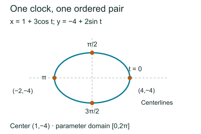One shared parameter synchronizes horizontal and vertical position. For x = 1 + 3 cos t and y = −4 + 2 sin t, increasing t traces the ellipse counterclockwise.

SECTION 4

Mathematical Framework

The mathematical foundation of parametric planar motion rests on defining two coordinate functions over a shared domain of the parameter. Below are the key equations and relationships you need to master for the AP Precalculus exam. We begin with the general form and then examine the most important special cases: linear motion, projectile motion, and circular (trigonometric) motion.

GENERAL PARAMETRIC FORM

x = f(t), y = g(t), t ∈ [a, b]

Here f and g are real-valued functions of the parameter t, and [a, b] specifies the interval over which the curve is traced. Each value of t produces exactly one point (x, y) in the plane.

LINEAR PARAMETRIC MOTION

x = x₀ + at, y = y₀ + bt

This models a particle starting at (x₀, y₀) and moving with constant horizontal speed a and constant vertical speed b. Eliminating t yields the Cartesian line y − y₀ = (b/a)(x − x₀), provided a ≠ 0.

PROJECTILE MOTION

x = (v₀ cos θ)t, y = (v₀ sin θ)t − ½gt²

A classic application where t is time, v₀ is the initial speed, θ is the launch angle measured from the horizontal, and g is the acceleration due to gravity (≈ 9.8 m/s²). The horizontal coordinate grows linearly while the vertical coordinate follows a quadratic, producing a parabolic trajectory.

CIRCULAR / ELLIPTICAL MOTION

x = h + a cos t, y = k + b sin t

When a = b = r, this traces a circle of radius r centered at (h, k). When a ≠ b, the curve is an ellipse with semi-major and semi-minor axes a and b. As t ranges from 0 to 2π, the curve is traversed exactly once counterclockwise.

Eliminating the Parameter

Converting from parametric to Cartesian form is a critical skill. The strategy depends on the type of functions involved. For polynomial parametric equations, you solve one equation for t algebraically and substitute into the other. For trigonometric parametric equations such as x = a cos t and y = b sin t, you use the Pythagorean identity cos²t + sin²t = 1. Rewriting gives (x/a)² + (y/b)² = 1, revealing the ellipse in standard form. It is essential to remember that elimination discards information about the parameter's domain and the direction of traversal; two different parametrizations can produce the same Cartesian equation while tracing different portions of the curve or moving in opposite directions.

💡

Exam Tip

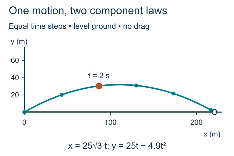When eliminating the parameter, always check whether the domain of t restricts the Cartesian curve. For example, x = t² and y = t⁴ yield y = x², but since x = t² ≥ 0 for all real t, only the right half of the parabola is actually traced.

An authored equal-scale trajectory diagram shows a ball above level ground, equally spaced horizontal sample positions and a highlighted point at two seconds, with no launching apparatus. A ball launched at 50 m/s at 30° has constant horizontal velocity and downward acceleration of 9.8 m/s². Equal-time points show equal horizontal steps and changing vertical steps.

SECTION 5

Types of Parametric Curves in Detail

Parametric curves encountered in AP Precalculus fall into several recognizable families. Understanding these families allows you to quickly identify the shape of a curve from its parametric equations, anticipate properties like symmetry and periodicity, and select the most efficient elimination strategy. The diagram below compares the four most common types side by side.

The four most common parametric curve families in AP Precalculus. Each panel shows the general shape, representative parametric equations, and a starting point at t = 0. The comparison table summarizes how they differ in Cartesian form, elimination strategy, closure, and periodicity.

Of these four families, the circular and elliptical cases are especially important on the AP exam because they involve trigonometric parametric equations and require the Pythagorean identity for elimination. Be attentive to the signs and coefficients: swapping cosine and sine, or negating one of them, changes both the starting point and the direction of traversal. For instance, x = r sin t and y = r cos t traces the same circle as x = r cos t and y = r sin t, but it begins at (0, r) instead of (r, 0) and traverses clockwise rather than counterclockwise.

SECTION 6

Worked Example

Let us work through a complete problem that ties together parametric representation, elimination, and analysis of motion.

Analyzing an Elliptical Parametric Curve

1
Step 1 — State the Problem

A particle moves in the xy-plane according to x(t) = 3 cos t + 1 and y(t) = 2 sin t − 4, for 0 ≤ t ≤ 2π. Determine the Cartesian equation of the curve, identify its shape and center, and describe the direction of motion.
2
Step 2 — Isolate the Trigonometric Expressions

From x(t) = 3 cos t + 1, subtract 1 from both sides to get x − 1 = 3 cos t, then divide: cos t = (x − 1)/3. Similarly, from y(t) = 2 sin t − 4, add 4 to both sides: y + 4 = 2 sin t, yielding sin t = (y + 4)/2.

cos t = (x − 1)/3, sin t = (y + 4)/2
3
Step 3 — Apply the Pythagorean Identity

Since cos²t + sin²t = 1, substitute the expressions from Step 2: [(x − 1)/3]² + [(y + 4)/2]² = 1. This simplifies to (x − 1)²/9 + (y + 4)²/4 = 1.

(x − 1)²/9 + (y + 4)²/4 = 1
4
Step 4 — Identify the Curve

This is the standard form of an ellipse centered at (h, k) = (1, −4) with semi-major axis a = 3 (horizontal, since 9 > 4) and semi-minor axis b = 2 (vertical). The vertices along the major axis are at (−2, −4) and (4, −4), while the co-vertices are at (1, −2) and (1, −6).

Ellipse centered at (1, −4) with a = 3, b = 2
5
Step 5 — Determine Direction and Starting Point

At t = 0: x(0) = 3 cos 0 + 1 = 4 and y(0) = 2 sin 0 − 4 = −4, so the particle starts at the right vertex (4, −4). At t = π/2: x(π/2) = 3(0) + 1 = 1 and y(π/2) = 2(1) − 4 = −2, placing the particle at the top co-vertex (1, −2). Since the particle moves from the right vertex to the top, the motion is counterclockwise. The full ellipse is traced exactly once as t goes from 0 to 2π.

Starts at (4, −4); traverses counterclockwise; one complete revolution on [0, 2π]

SECTION 7

Strengths, Limitations, and Comparisons

Parametric functions are a powerful tool, but like any mathematical representation, they have both advantages and limitations when compared with the standard Cartesian and polar representations. Understanding when to deploy each representation is part of developing mathematical fluency.

Feature	Parametric	Cartesian y = f(x)	Polar r = f(θ)
Can model non-function curves	Yes — loops, crossings, vertical lines	No — fails vertical line test	Yes — many polar curves are non-functions in Cartesian
Encodes direction of motion	Yes — inherent in increasing t	No — purely geometric	Yes — via increasing θ
Encodes speed / timing	Yes — different parametrizations vary speed	No	Partially — rate of angle change
Ease of graphing by hand	Moderate — requires a t-table	Easy — plot points or use transformations	Moderate — requires angle-radius table
Best suited for	Motion modeling, animation, complex curves	Single-valued relationships, function analysis	Symmetric curves centered at the origin

Comparison of curve representations

✦

KEY TAKEAWAY

Parametric, Cartesian, and polar representations are like three different languages describing the same geometric object. Each language has its own grammar and strengths. Parametric is the language of motion and engineering—it tells you not just where the path is, but when and how fast an object traverses it. Choose your representation based on what question you are trying to answer: shape alone calls for Cartesian, symmetry around a center calls for polar, and anything involving time or directed traversal calls for parametric.

SECTION 8

Connections to Advanced Topics

Parametric functions modeling planar motion serve as a gateway to several advanced mathematical and scientific topics. In AP Calculus BC, you will compute derivatives and integrals of parametric curves—finding tangent slopes via dy/dx = (dy/dt)/(dx/dt), computing arc lengths, and determining enclosed areas. In multivariable calculus, parametric descriptions generalize to vector-valued functions r(t) = ⟨x(t), y(t), z(t)⟩ in three-dimensional space, forming the basis for studying space curves, curvature, and the motion of objects in three dimensions.

AP Precalculus Topic	Advanced Extension
Parametric equations x(t), y(t)	Vector-valued functions r(t) = ⟨x(t), y(t)⟩ in Calculus BC and multivariable calculus
Eliminating the parameter to find Cartesian form	Implicit differentiation of the resulting Cartesian equation
Direction of motion (orientation)	Velocity and acceleration vectors v(t) = r′(t), a(t) = r″(t)
Circular motion x = r cos t, y = r sin t	Uniform circular motion in physics: centripetal acceleration, angular velocity
Projectile parametric equations	Differential equations of motion with drag, variable gravity, and three-dimensional trajectories

From AP Precalculus to advanced coursework

The conceptual leap from parametric functions to vector-valued functions is remarkably small: where AP Precalculus treats x(t) and y(t) as separate equations, calculus bundles them into a single vector r(t). This shift in notation opens the door to computing tangent vectors, normal vectors, and curvature—tools that underpin modern physics, computer-aided design, and robotics. Mastering parametric thinking now positions you to transition smoothly into these more advanced frameworks.

SECTION 9

Practice Problems

Question 1: CONCEPTUAL

A particle moves in the xy-plane with parametric equations x(t) = 2t + 1 and y(t) = 5 − t for t ≥ 0. Which of the following best describes why the parametric representation provides more information than the Cartesian equation of the same curve?

A. The parametric form shows that the curve is a line, which cannot be determined from the Cartesian equation.
B. The parametric form specifies the direction of motion and the starting point, which the Cartesian equation does not.
C. The parametric form allows the curve to pass the vertical line test, while the Cartesian form does not.
D. The parametric form produces a different curve than the Cartesian equation derived from it.
E. The parametric form is required because the Cartesian equation cannot be obtained by eliminating t.

Show answer (B)

B is correct. Eliminating t from x = 2t + 1 and y = 5 − t yields the Cartesian equation y = −½x + 5.5, which describes a line. However, this Cartesian equation alone does not tell us that the particle starts at (1, 5) when t = 0, nor that it moves to the right and downward as t increases—the parametric form encodes both the starting point and direction. A is wrong because the Cartesian equation also shows the curve is a line. C is wrong because this particular Cartesian equation does pass the vertical line test. D is wrong because the parametric and Cartesian forms describe the same geometric path (though the parametric form only traces the ray for t ≥ 0). E is wrong because t is easily eliminated by solving for t in either equation.

Question 2: BASIC CALCULATION

A particle moves according to x(t) = 4 cos t and y(t) = 4 sin t for 0 ≤ t ≤ 2π. What is the Cartesian equation of the path, and what are the coordinates of the particle at t = π/3?

A. x² + y² = 16; particle at (2, 2√3)
B. x² + y² = 4; particle at (2, 2√3)
C. x² + y² = 16; particle at (2√3, 2)
D. x² + y² = 16; particle at (−2, 2√3)
E. x² + y² = 8; particle at (2√2, 2√2)

Show answer (A)

A is correct. Using cos²t + sin²t = 1, we get (x/4)² + (y/4)² = 1, so x² + y² = 16—a circle of radius 4 centered at the origin. At t = π/3: x = 4 cos(π/3) = 4(½) = 2 and y = 4 sin(π/3) = 4(√3/2) = 2√3, giving (2, 2√3). B is wrong because the radius is 4, not 2, so the equation is x² + y² = 16, not 4. C incorrectly swaps the x and y coordinates. D has the wrong sign on the x-coordinate; cos(π/3) = ½ > 0. E uses incorrect values that correspond to t = π/4 on a circle of radius 2√2.

Question 3: INTERMEDIATE

Given the parametric equations x(t) = t² − 2t and y(t) = t + 1 for all real t, which of the following is the correct Cartesian equation after eliminating the parameter?

A. x = y² − 4y + 3
B. x = y² − 2y + 1
C. x = y² + 4y − 3
D. y = x² − 2x + 1
E. x = y² − 1

Show answer (A)

A is correct. From y = t + 1, solve for t: t = y − 1. Substitute into x = t² − 2t to get x = (y − 1)² − 2(y − 1) = y² − 2y + 1 − 2y + 2 = y² − 4y + 3. B is wrong because it only computes (y − 1)² = y² − 2y + 1 without subtracting 2(y − 1). C has the wrong signs on the linear and constant terms. D incorrectly writes y as a function of x with a different expression entirely. E oversimplifies the algebra and omits the linear term.

Question 4: APPLIED

4 pts

A projectile is launched from the origin at an initial speed of 50 m/s at an angle of 30° above the horizontal. The parametric equations of its motion are x(t) = (50 cos 30°)t and y(t) = (50 sin 30°)t − 4.9t². (a) Find the exact parametric equations using the known values of cos 30° and sin 30°. (b) Determine the time at which the projectile reaches its maximum height, and find that maximum height. (c) Find the total horizontal distance (range) the projectile travels before returning to ground level. (d) Eliminate the parameter to write y as a function of x, and identify the shape of the trajectory.

Show answer

Point 1 (1 pt): Part (a). cos 30° = √3/2 and sin 30° = 1/2, so x(t) = 25√3 · t and y(t) = 25t − 4.9t². Award 1 point for correctly substituting both trigonometric values. Point 2 (1 pt): Part (b). Maximum height occurs when dy/dt = 0. Since dy/dt = 25 − 9.8t, setting this to zero gives t = 25/9.8 ≈ 2.551 s. Maximum height: y(25/9.8) = 25(25/9.8) − 4.9(25/9.8)² = 625/9.8 − 4.9(625/96.04) = 625/9.8 − 3062.5/96.04 ≈ 63.78 − 31.89 ≈ 31.89 m. Equivalently, y_max = 25²/(2 × 4.9) = 625/9.8 ≈ 31.89 m. Award 1 point for correct time and maximum height. Point 3 (1 pt): Part (c). The projectile returns to ground level when y(t) = 0: 25t − 4.9t² = 0 → t(25 − 4.9t) = 0, giving t = 0 (launch) or t = 25/4.9 ≈ 5.102 s. Range: x(25/4.9) = 25√3 · (25/4.9) = 625√3/4.9 ≈ 220.92 m. Award 1 point for correct landing time and range. Point 4 (1 pt): Part (d). From x = 25√3 · t, solve t = x/(25√3). Substitute: y = 25 · x/(25√3) − 4.9 · x²/(625 · 3) = x/√3 − 4.9x²/1875 = (√3/3)x − (4.9/1875)x². This is a quadratic in x (downward-opening parabola) confirming a parabolic trajectory. Award 1 point for correct elimination and identification of the parabola.

Question 5: CRITICAL THINKING

3 pts

Consider two parametrizations of the same curve: Parametrization I: x₁(t) = cos t, y₁(t) = sin t, 0 ≤ t ≤ π Parametrization II: x₂(t) = 1 − 2t², y₂(t) = 2t√(1 − t²), 0 ≤ t ≤ 1 (a) Show that both parametrizations trace the same Cartesian curve. (b) Determine the starting and ending points for each, and compare the directions of traversal. (c) Explain, in general terms, why infinitely many different parametrizations can represent the same geometric curve, and discuss what distinguishes one parametrization from another.

Show answer

Point 1 (1 pt): Part (a). For Parametrization I: cos²t + sin²t = 1, so x₁² + y₁² = 1, which is the unit circle. For Parametrization II: x₂² + y₂² = (1 − 2t²)² + (2t√(1 − t²))² = 1 − 4t² + 4t⁴ + 4t²(1 − t²) = 1 − 4t² + 4t⁴ + 4t² − 4t⁴ = 1. So x₂² + y₂² = 1 as well. Both trace the unit circle. Award 1 point for verifying x² + y² = 1 for both parametrizations. Point 2 (1 pt): Part (b). Parametrization I: At t = 0, (cos 0, sin 0) = (1, 0). At t = π, (cos π, sin π) = (−1, 0). The upper semicircle is traced counterclockwise from (1, 0) to (−1, 0). Parametrization II: At t = 0, (1 − 0, 0) = (1, 0). At t = 1, (1 − 2, 0) = (−1, 0). For 0 < t < 1, y₂(t) = 2t√(1 − t²) > 0, so the particle is in the upper half-plane. Both trace the upper semicircle from (1, 0) to (−1, 0) in the same counterclockwise direction, but at different speeds. Award 1 point for correct endpoints and direction comparison. Point 3 (1 pt): Part (c). Infinitely many parametrizations exist because any continuous, monotonic reparametrization s = φ(t) applied to a valid parametrization produces another valid one tracing the same curve. What distinguishes one from another is the relationship between the parameter and position: different parametrizations assign different speeds to the traversal, different starting points, or even different directions. The geometric locus is the same, but the kinematic information—when each point is visited and how fast—varies. Award 1 point for a clear explanation referencing reparametrization and the distinction between geometric and kinematic content.

SUMMARY

Lesson Summary

Summary

Parametric functions model planar motion by expressing the coordinates x and y as separate functions of a shared parameter t. Unlike a Cartesian equation y = f(x), a parametric representation captures not only the shape of a curve but also the direction of motion and the rate at which the curve is traversed. The key families include linear (x = x₀ + at, y = y₀ + bt), projectile / parabolic, and circular / elliptical (x = a cos t, y = b sin t) parametrizations.

To convert from parametric to Cartesian form, you eliminate the parameter either by algebraic substitution or by invoking the Pythagorean identity cos²t + sin²t = 1 for trigonometric cases. Always check whether the domain of t restricts the Cartesian curve to a subset. Mastering parametric functions builds the foundation for vector-valued functions and calculus-based motion analysis in more advanced courses.