Matrices Modeling Contexts - AP Precalculus

SECTION 1

Historical Context & Motivation

Long before digital computers, mathematicians and scientists needed compact ways to represent and manipulate systems of equations that arose in surveying, astronomy, and commerce. The idea of arranging coefficients into a rectangular grid—what we now call a matrix—evolved over centuries, driven by the practical need to solve multiple simultaneous linear equations without rewriting every variable each time. The concept matured in the nineteenth century when algebraists realized that the array itself, independent of any particular system, carried rich structural information that could model economic transactions, geometric transformations, and network relationships.

~200 BCE • Chinese 'Fangcheng' Method

The Chinese text Nine Chapters on the Mathematical Art presented a rectangular tableau of coefficients to solve systems of linear equations, anticipating Gaussian elimination by nearly two millennia.

1850 • Sylvester Coins 'Matrix'

James Joseph Sylvester introduced the term matrix (Latin for 'womb') to describe a rectangular array from which determinants could be formed.

1858 • Cayley Formalizes Matrix Algebra

Arthur Cayley published A Memoir on the Theory of Matrices, defining addition, multiplication, and the identity and inverse matrices, thereby establishing the algebraic framework still used today.

1949 • Leontief's Input–Output Model

Wassily Leontief used matrices to model how industries in an economy supply one another, winning the Nobel Prize in Economics and demonstrating the power of matrices in applied contexts.

2000s • Matrices in Data Science & AI

Modern machine-learning algorithms store data in massive matrices, and operations such as matrix factorization underpin recommendation engines, image recognition, and natural language processing.

This historical trajectory reveals the central question that drives the present lesson: how can a single rectangular array of numbers faithfully represent—and allow us to compute with—a wide variety of real-world situations, from tracking inventory across multiple stores to describing the connectivity of a social network? Answering this question equips you with one of the most versatile modeling tools in precalculus and beyond.

SECTION 2

Core Principles & Definitions

A matrix is a rectangular array of numbers organized into rows and columns, enclosed in brackets. Each individual number is called an element (or entry), and the position of an element is specified by its row number and column number. A matrix with m rows and n columns is said to have dimensions (or order) m × n. Understanding these structural properties is essential before exploring how matrices model real-world contexts, because the dimensions of a matrix carry semantic meaning: the rows typically correspond to one category (e.g., stores), while the columns correspond to another (e.g., products).

Dimensions Carry Meaning

In a contextual matrix, rows and columns represent distinct real-world categories. A 3 × 4 matrix might encode 3 factories producing 4 products, so the dimensions themselves are part of the model.

Elements Encode Data

Each entry aᵢⱼ stores a single datum—price, distance, probability, or quantity—linked to row i and column j. The positional notation ensures that data retrieval is unambiguous.

Matrix Operations Correspond to Real Actions

Adding two matrices models combining inventories; multiplying a matrix by a scalar models applying a uniform percentage change; matrix multiplication chains two relationships together.

Compatibility Rules Prevent Nonsense

Two matrices can be added only when they share the same dimensions, and the product AB exists only when the number of columns of A equals the number of rows of B—ensuring the 'inner categories' align.

✦

KEY TAKEAWAY

Think of a matrix like a spreadsheet tab: the row headers and column headers describe what each entry means, while the grid of numbers stores the actual data. Matrix operations are the algebraic equivalent of writing formulas that span multiple cells—addition merges two tabs, scalar multiplication adjusts every cell uniformly, and matrix multiplication cross-references one tab against another to compute a derived result, much as a VLOOKUP chains two tables.

SECTION 3

Visual Explanation — Matrices as Data Tables

The inventory matrix A has 3 rows (one per store) and 4 columns (one per product). Each entry a_ij tells us how many units of product j are held at store i.

The diagram above illustrates the most fundamental idea of this lesson: a matrix is not simply an abstract mathematical object but rather a structured model of a real situation. Each row header labels a category (here, a retail store), each column header labels a second category (a product), and the entry at their intersection records the datum that links them. When you encounter a contextual matrix problem on the AP Precalculus exam, your first task is always to identify what the rows represent and what the columns represent; from there, the meaning of every element and every operation follows naturally.

SECTION 4

Mathematical Framework — Operations in Context

Three matrix operations appear consistently in AP Precalculus modeling problems: matrix addition, scalar multiplication, and matrix multiplication. Each operation has precise dimensional requirements and a clear contextual interpretation. Understanding these requirements not only prevents computational errors but also deepens your insight into why certain real-world combinations of data are meaningful while others are not.

MATRIX ADDITION

A + B = [aᵢⱼ + bᵢⱼ] (same dimensions m × n required)

If A and B are both m × n matrices, their sum is the m × n matrix formed by adding corresponding entries. Context: combining inventories from two months, or totaling points from two games.

SCALAR MULTIPLICATION

kA = [k · aᵢⱼ] (k ∈ ℝ)

Every entry of A is multiplied by the scalar k. Context: a 10% price increase corresponds to multiplying a price matrix by 1.10; halving production corresponds to multiplying by 0.5.

MATRIX MULTIPLICATION

(AB)ᵢⱼ = Σₖ aᵢₖ · bₖⱼ (A is m × p, B is p × n → AB is m × n)

Entry (i, j) of the product AB is the dot product of the i-th row of A and the j-th column of B. The inner dimension p must match. Context: multiplying a quantity matrix by a unit-price column vector yields total costs.

💡

Dimension Compatibility Tip

When computing AB, write the dimensions side by side: (m × p)( p × n). The two bold inner numbers must agree; the outer numbers give the dimensions of the result. In a modeling context, the shared inner dimension is the category being 'summed over'—for example, products, when quantity-per-store is multiplied by price-per-product.

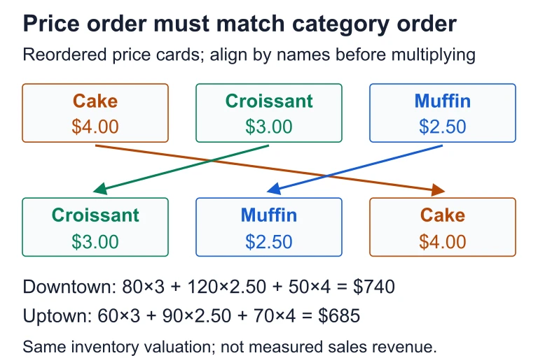
Two bakery counter sections display croissants,muffins and cakes while the exact matrix matches inventory quantities to the same price categories. Align the product categories in each inventory row with the same categories in the price column. Their dot product gives the value of that location’s inventory.

Align the product categories in each inventory row with the same categories in the price column. Their dot product gives the value of that location’s inventory.

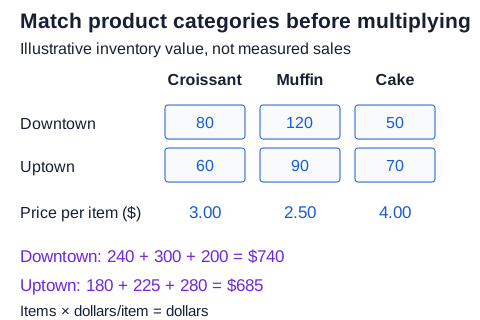
Inventory table for Downtown and Uptown lists croissants, muffins and cakes and multiplies the aligned quantities by prices to produce $740 and $685. For croissants, muffins and cakes priced at $3, $2.50 and $4, the inventory rows (80, 120, 50) and (60, 90, 70) give values $740 and $685. Each row’s quantities pair with the same product order in the price column.Open full diagram

SECTION 5

Common Modeling Contexts

Matrices arise in a surprisingly broad range of applied settings. On the AP Precalculus exam, you are most likely to encounter matrices that model business data (inventory, cost, revenue), transition processes (population movement, probability), or network connectivity. Below is a classification of the most common contexts, followed by a diagram that illustrates how matrix multiplication chains two relationships.

Context Type	Rows Represent	Columns Represent	Entries Represent
Inventory / Production	Stores or factories	Products	Quantities
Cost / Revenue	Products	Cost categories (price, tax)	Dollar amounts
Transition / Markov	Current state	Next state	Probabilities
Network / Adjacency	Nodes (cities, people)	Nodes (cities, people)	1 (connected) or 0 (not)
Nutrition / Composition	Foods or recipes	Nutrients	Grams or milligrams per serving

Five common matrix-modeling contexts encountered in AP Precalculus.

The Quantity matrix Q (3 × 4) multiplied by the Price column vector P (4 × 1) produces the Revenue vector R (3 × 1). The shared inner dimension—4 products—is 'summed over,' yielding one total revenue figure per store.

The diagram above crystallizes the central idea behind matrix multiplication in a modeling context. The quantity matrix and the price vector share the 'products' category as their inner dimension, and the multiplication sums over products to produce a total revenue for each store. This pattern—chain two related tables by their shared category—generalizes to any pair of compatible matrices, whether you are computing total calories per meal from servings-per-ingredient and calories-per-ingredient, or computing expected populations from current populations and transition probabilities.

SECTION 6

Worked Example — Business Revenue Calculation

A bakery operates two locations, Downtown (D) and Uptown (U). Each location sells three products: Croissants, Muffins, and Scones. The number of each item sold on a given day is recorded in the matrix S, and the unit price of each item is given in the column vector P. Find the total revenue for each location.

Computing Daily Revenue by Location

1
Step 1 — Identify the Matrices and Their Meaning

Sales matrix S (2 × 3): rows are locations {D, U}, columns are products {Croissants, Muffins, Scones}. S = [ 80 120 50 ; 60 90 70 ]. Price column P (3 × 1): rows are products, P = [ $3.00 ; $2.50 ; $4.00 ].

S is 2 × 3, P is 3 × 1 → product SP will be 2 × 1.
2
Step 2 — Verify Dimensional Compatibility

The number of columns in S (3 products) equals the number of rows in P (3 products). The inner dimensions match, so the multiplication is defined. The result will have 2 rows (locations) and 1 column—a revenue total for each location.

Inner dimension = 3 ✓. Result: 2 × 1 matrix.
3
Step 3 — Compute Entry (1, 1): Downtown Revenue

Take the dot product of row 1 of S and column 1 of P: 80 × $3.00 + 120 × $2.50 + 50 × $4.00 = $240 + $300 + $200 = $740.

Downtown revenue = $740
4
Step 4 — Compute Entry (2, 1): Uptown Revenue

Take the dot product of row 2 of S and column 1 of P: 60 × $3.00 + 90 × $2.50 + 70 × $4.00 = $180 + $225 + $280 = $685.

Uptown revenue = $685
5
Step 5 — State the Result Matrix

The revenue matrix R = SP = [ $740 ; $685 ]. This 2 × 1 column vector tells us each location's daily revenue in a single, compact matrix.

R = [ 740 ; 685 ]

SECTION 7

Strengths & Limitations of Matrix Models

Strengths	Limitations
Compact representation of large data sets; a single symbol can encode hundreds of values.	Dimensional constraints mean not every pair of matrices can be combined—real-world data must be organized carefully.
Operations (addition, multiplication) directly mirror real actions (combining, chaining), making models interpretable.	Matrix multiplication is not commutative (AB ≠ BA in general), so the order of factors must match the direction of the real-world relationship.
Scales to very large systems via computer implementation; identical algebra works for 2 × 2 and 200 × 200 matrices.	Entries must share a common unit within each matrix; mixing dollars and percentages in the same array produces meaningless results.
Provides a bridge to linear algebra, enabling eigenvalue analysis, least-squares fitting, and systems of equations.	Only models linear relationships; nonlinear interactions (e.g., economies of scale) require extensions beyond basic matrix arithmetic.

Strengths and limitations of using matrices to model real-world contexts.

✦

KEY TAKEAWAY

A matrix model is like an engineering blueprint: it captures the essential structural relationships—dimensions, connections, quantities—while deliberately omitting details (color, texture, emotion) that lie outside its scope. Just as a blueprint is powerful precisely because it simplifies, a matrix model is powerful because it distills a complex system into a grid of numbers that can be manipulated algebraically. The trade-off is that the model is only as faithful as the assumptions built into its rows and columns.

SECTION 8

Connection to Advanced Theory

In AP Precalculus, you use matrices primarily to store data and perform arithmetic operations that correspond to real-world computations. In college-level linear algebra and beyond, the same matrix framework opens the door to far more sophisticated techniques. The table below previews how each precalculus concept extends into advanced territory.

AP Precalculus Concept	Advanced Extension
Matrix as a data table	Matrices as linear transformations acting on vector spaces; eigenvectors reveal the transformation's 'principal axes.'
Matrix multiplication chains two relationships	Composition of linear maps; Markov chains use repeated matrix multiplication (Aⁿ) to forecast long-run state distributions.
Scalar multiplication scales all entries	Eigenvalues generalize scalar multiplication to specific directions; diagonalization decomposes A = PDP⁻¹.
Dimensional compatibility rules	Rank-nullity theorem and the study of kernel/image provide deeper reasons why certain systems have solutions.
Inverse matrix solving Ax = b	LU decomposition, QR factorization, and singular value decomposition (SVD) solve larger, more numerically sensitive systems.

How AP Precalculus matrix concepts connect to linear algebra.

Recognizing these connections is not required for the AP exam, but it can deepen your appreciation for why the exam emphasizes dimensional reasoning, contextual interpretation, and the non-commutativity of matrix multiplication. Every skill you build now transfers directly into the more powerful toolkit of linear algebra.

SECTION 9

Practice Problems

Question 1: CONCEPTUAL

A matrix M has dimensions 5 × 3. In a business context, the rows of M represent five different warehouses and the columns represent three different products. What does the entry m₂₃ represent?

A. The total number of products stored across all warehouses
B. The quantity of product 3 stored at warehouse 2
C. The quantity of product 2 stored at warehouse 3
D. The total inventory at warehouse 2
E. The price of product 3

Show answer (B)

The correct answer is B. In the subscript notation mᵢⱼ, the first subscript i identifies the row and the second subscript j identifies the column. Since rows represent warehouses and columns represent products, m₂₃ specifies the datum at warehouse 2 (row 2) and product 3 (column 3): the quantity of product 3 stored at warehouse 2. Choice A is wrong because it describes a sum across all warehouses, which is not a single entry but a column sum. Choice C reverses the subscript order; m₂₃ ≠ m₃₂. Choice D describes the sum of an entire row, not a single entry. Choice E confuses the matrix with a different matrix (a price matrix) entirely.

Question 2: BASIC CALCULATION

A coffee shop tracks daily sales in the matrix S = [ 40 25 ; 55 30 ], where rows are {Morning, Afternoon} and columns are {Lattes, Teas}. If lattes sell for $5 each and teas sell for $3 each, the price column vector is P = [ 5 ; 3 ]. What is the total morning revenue?

A. $195
B. $275
C. $365
D. $200
E. $325

Show answer (B)

The correct answer is B. Morning revenue is the dot product of row 1 of S with column vector P: 40 × $5 + 25 × $3 = $200 + $75 = $275. Choice A ($195) might result from mistakenly using the afternoon row (55 × 3 + 30 × ... — a miscalculation). Choice C ($365) equals the sum of morning and afternoon revenue for lattes only (40 + 55) × 5 = 475, not matching either, and represents a misapplication. Choice D ($200) only accounts for latte revenue and ignores teas. Choice E ($325) is the afternoon revenue (55 × 5 + 30 × 3 = 275 + 90 = 365 — actually $365, so $325 is simply a distractor that matches no valid computation).

Question 3: INTERMEDIATE

Matrix A (3 × 4) represents the number of units produced by 3 factories for 4 models, matrix B (4 × 2) gives the raw-material cost and labor cost per unit for each of the 4 models, and matrix C (2 × 1) gives the markup factor for each cost category (raw materials and labor). A student wants to compute a single matrix that gives the total production cost per factory. Which expression is dimensionally defined and produces a 3 × 1 result matrix with the correct interpretation?

A. A(BC)
B. B(AC)
C. CBA
D. BAC
E. A + B + C

Show answer (A)

We need to find which expression is dimensionally defined AND produces a 3 × 1 matrix with the correct interpretation (total production cost per factory). Choice A: A(BC). BC is (4 × 2)(2 × 1) = 4 × 1 (total cost per unit for each model). Then A(BC) is (3 × 4)(4 × 1) = 3 × 1 (total production cost per factory). Dimensions work and interpretation is correct. Choice B: B(AC). AC requires (3 × 4)(2 × 1). Columns of A (4) ≠ rows of C (2), so AC is undefined. This expression is invalid. Choice C: CBA. CB requires (2 × 1)(4 × 2). Columns of C (1) ≠ rows of B (4), so CB is undefined. This expression is invalid. Choice D: BAC. BA requires (4 × 2)(3 × 4). Columns of B (2) ≠ rows of A (3), so BA is undefined. This expression is invalid. Choice E: A + B + C. Addition requires all matrices to have the same dimensions. A is 3 × 4, B is 4 × 2, and C is 2 × 1, so addition is undefined. The correct answer is A.

Question 4: APPLIED

4 pts

A school district has two high schools, North and South. Each school's students are classified by grade level (10th, 11th, 12th) and activity preference (Sports, Arts, STEM). The enrollment data is given by the matrix E, and the per-student funding for each activity is given by the vector F. E (2 × 3 — schools × activities): North: [ 300 150 250 ] South: [ 220 180 200 ] F (3 × 1 — activities × dollars): [ $120 ] [ $200 ] [ $180 ] (a) State the dimensions of the product EF and explain what each entry represents in context. (b) Compute EF. (c) The district receives a 15% budget increase for all activities. Write a matrix expression using scalar multiplication that computes the new total funding per school, and evaluate it. (d) If the district wanted to compare total funding across all three activities for both schools side by side—rather than as a single total per school—which matrix product would provide a 2 × 3 result showing funding per school per activity? Explain.

Show answer

Rubric (4 points): Point 1 — Part (a): EF has dimensions (2 × 3)(3 × 1) = 2 × 1. Each entry represents the total activity funding for one school: entry (1,1) = North's total funding, entry (2,1) = South's total funding. Point 2 — Part (b): North funding = 300(120) + 150(200) + 250(180) = 36,000 + 30,000 + 45,000 = $111,000. South funding = 220(120) + 180(200) + 200(180) = 26,400 + 36,000 + 36,000 = $98,400. EF = [ 111,000 ; 98,400 ]. Point 3 — Part (c): New funding = 1.15 × EF = 1.15 × [ 111,000 ; 98,400 ] = [ 127,650 ; 113,160 ]. The scalar 1.15 multiplies every entry of EF, reflecting the uniform 15% increase. Point 4 — Part (d): To obtain a 2 × 3 result showing funding per school per activity, you need each entry to equal (enrollment in activity j at school i) × (funding per student for activity j). This is achieved by element-wise multiplication (Hadamard product) or equivalently by E × diag(F), where diag(F) is the 3 × 3 diagonal matrix with the entries of F on the diagonal: diag(120, 200, 180). Then E × diag(F) is (2 × 3)(3 × 3) = 2 × 3, and entry (i, j) = eᵢⱼ × fⱼ, which is the total activity-j funding at school i.

Question 5: CRITICAL THINKING

3 pts

Consider two matrices: M (n × n) is a transition matrix where mᵢⱼ represents the fraction of the population that moves from city j to city i each year, and v (n × 1) is a column vector representing the current population of each city. (a) Explain in context what the product Mv represents. (b) Explain in context what the product M²v = M(Mv) represents. (c) A student claims that the product vM would give the same information as Mv. Is this claim correct? Justify your answer using dimensional analysis and contextual reasoning.

Show answer

Rubric (3 points): Point 1 — Part (a): The product Mv is an n × 1 vector whose i-th entry equals the sum mᵢ₁v₁ + mᵢ₂v₂ + … + mᵢₙvₙ. This represents the predicted population of city i after one year, obtained by summing the fractions of each city's population that migrate to city i. Point 2 — Part (b): M²v = M(Mv) applies the transition matrix twice. First, Mv gives the population distribution after one year; then multiplying by M again gives the distribution after two years. This models two successive years of migration under the same transition probabilities. Point 3 — Part (c): The claim is incorrect. v is n × 1 and M is n × n; the product vM would require v to have as many columns as M has rows, but v has only 1 column while M has n rows, so vM is dimensionally undefined (1-column matrix cannot left-multiply an n-row matrix unless n = 1). Even if one attempted vᵀM (a 1 × n times n × n = 1 × n product), the resulting row vector would have a different contextual meaning: entry j of vᵀM would sum populations weighted by the fractions leaving for city j, which mixes rows and columns of M in a way that does not represent next-year populations in the same sense as Mv. The non-commutativity of matrix multiplication means the order encodes the direction of the relationship.

SUMMARY

Lesson Summary

Summary

A matrix is a rectangular array of numbers whose rows and columns correspond to real-world categories such as stores, products, cities, or nutrients. Each element aᵢⱼ encodes a datum linking the row-i category to the column-j category. The three essential operations—matrix addition (combining same-structure data), scalar multiplication (uniform scaling), and matrix multiplication (chaining two relationships via a shared inner dimension)—each have direct contextual interpretations.

When approaching any AP Precalculus matrix problem, begin by identifying what the dimensions represent, verify dimensional compatibility before computing, and interpret the resulting matrix in the language of the original context. Remember that matrix multiplication is not commutative: the order of factors encodes the direction of the relationship being modeled. Mastering these principles positions you both for exam success and for the richer world of linear algebra that lies ahead.