

SECTION 1
Historical Context & Motivation
The concept of rate of change lies at the very heart of mathematics and the physical sciences, providing the formal language for describing how one quantity responds to shifts in another. Long before the machinery of calculus was available, mathematicians and natural philosophers recognized that understanding motion, growth, and geometric form required more than static measurement—it demanded a way to capture how quickly things change. From ancient Greek investigations of area and slope to the Renaissance's kinematic breakthroughs, the evolution of rate-of-change thinking laid the groundwork for modern analysis. In the AP Precalculus framework, mastering rates of change in linear and quadratic functions forms an essential bridge: it connects algebraic structure to the dynamic, function-behavior perspective that pervades higher mathematics.
c. 300 BCE • Euclid and Proportional Change
c. 1638 • Galileo's Kinematic Laws
1637 • Descartes and Analytic Geometry
1665–1687 • Newton and Leibniz — The Calculus
2023–present • AP Precalculus Curriculum
The central question this lesson addresses is deceptively simple: How does the output of a function change as its input changes, and what does the pattern of that change reveal about the function's type? For linear functions, the answer is a single constant; for quadratic functions, the answer is itself a linear function—a fact with deep structural implications that foreshadow the derivative in calculus.
SECTION 2
Core Principles & Definitions
Before diving into computation, it is essential to establish the foundational ideas that govern rates of change across function families. The average rate of change (AROC) of a function f over an interval [a, b] measures the ratio of the change in output to the change in input: Δf / Δx = (f(b) − f(a)) / (b − a). Geometrically, this is the slope of the secant line connecting the points (a, f(a)) and (b, f(b)) on the graph. The behavior of the AROC as the interval varies is what distinguishes one function family from another, and the four principles below capture the key structural insights needed for AP Precalculus.
Constant Rate of Change (Linear)
Variable Rate of Change (Quadratic)
Second Differences Are Constant
Secant vs. Tangent Interpretation
KEY TAKEAWAY
SECTION 3
Visual Explanation — Secant Lines and Slope Behavior
The diagram above crystallizes the fundamental distinction between linear and quadratic behavior. On the left, every secant line drawn on f(x) = 2x + 1 is parallel—they all have slope 2. This visual uniformity corresponds to the algebraic fact that the average rate of change is the same over every interval. On the right, secant lines drawn on g(x) = x² + 1 progressively steepen as we move to the right, with slopes following the odd-number pattern 1, 3, 5, 7, … for consecutive unit intervals. This increasing steepness is what produces curvature: the graph bends because the rate at which output grows is itself growing. Notice that the differences between consecutive AROC values (3 − 1 = 2, 5 − 3 = 2, 7 − 5 = 2) are constant—this constant second difference equals 2a where a = 1 is the leading coefficient of the quadratic.
SECTION 4
Mathematical Framework
We now formalize the rate-of-change relationships for linear and quadratic functions using algebraic derivations. These formulas appear frequently on the AP Precalculus exam and provide the computational backbone for both multiple-choice and free-response questions.
AVERAGE RATE OF CHANGE (GENERAL)
where f is any function, and [a, b] is the interval over which the change is measured. This quotient equals the slope of the secant line through (a, f(a)) and (b, f(b)).
AROC FOR A LINEAR FUNCTION f(x) = mx + b
Substituting f(x) = mx + b into the AROC formula: the constant term b cancels, and the factor (b₂ − a) cancels from numerator and denominator, leaving AROC = m for every interval. Note: here b₂ denotes the right endpoint to avoid confusion with the y-intercept b.
AROC FOR A QUADRATIC FUNCTION f(x) = ax² + bx + c
Derivation: f(x₂) − f(x₁) = a(x₂² − x₁²) + b(x₂ − x₁) = (x₂ − x₁)[a(x₂ + x₁) + b]. Dividing by (x₂ − x₁) yields AROC = a(x₂ + x₁) + b. This is a linear function of the endpoints, confirming that the rate of change of a quadratic function is itself linear.
SECOND DIFFERENCES (EQUALLY SPACED DATA)
When inputs are equally spaced by step h, the second difference of a quadratic f(x) = ax² + bx + c is always 2ah². This constant value is the hallmark test for quadratic behavior in tabular data. For unit spacing (h = 1), the second difference simplifies to 2a.
AP Exam Tip
SECTION 5
First Differences, Second Differences, and the Difference Table
One of the most practical tools for analyzing rates of change is the difference table, which organizes input–output data along with successive layers of differences. Given equally spaced inputs x₀, x₁, x₂, …, we define the first differences as Δf = f(xₙ₊₁) − f(xₙ), which are proportional to the AROC over each subinterval. The second differences are Δ²f = Δfₙ₊₁ − Δfₙ, and they measure how the rate of change itself changes. For a linear function, first differences are constant and second differences are zero. For a quadratic function, first differences are linear and second differences are constant.
The difference table makes the hierarchical structure of polynomial behavior immediately visible. For f(x) = 2x² − x + 3, the first differences 1, 5, 9, 13, 17 are not constant, so the function is not linear. However, the differences of these differences—4, 4, 4, 4—are constant, confirming that f is quadratic. This is the discrete analogue of the calculus fact that the second derivative of a quadratic is a constant. More generally, a polynomial of degree n has constant nth differences, and all higher differences are zero—a principle that extends the linear/quadratic distinction to cubics, quartics, and beyond.
SECTION 6
Worked Example — Identifying and Computing Rates of Change
Consider the function g(x) = −3x² + 12x − 5. We want to find the average rate of change on the interval [1, 4], determine the x-value where the instantaneous rate of change equals zero (the vertex), and verify the second-difference pattern from a table of values.
Finding the AROC and Interpreting Quadratic Behavior
- 1
Step 1 — Evaluate the function at the endpoints
Compute g(1) and g(4). We have g(1) = −3(1)² + 12(1) − 5 = −3 + 12 − 5 = 4 and g(4) = −3(4)² + 12(4) − 5 = −48 + 48 − 5 = −5.g(1) = 4, g(4) = −5 - 2
Step 2 — Apply the AROC formula
AROC = [g(4) − g(1)] / (4 − 1) = (−5 − 4) / 3 = −9 / 3 = −3. Alternatively, using the quadratic shortcut: AROC = a(x₁ + x₂) + b = −3(1 + 4) + 12 = −15 + 12 = −3. Both methods agree.AROC on [1, 4] = −3 - 3
Step 3 — Find the vertex (zero rate of change)
The vertex of g(x) = ax² + bx + c occurs at x = −b/(2a). Here, x = −12/(2 × (−3)) = −12/(−6) = 2. At x = 2, the instantaneous rate of change is zero, meaning the AROC over any interval centered at x = 2 (such as [2 − h, 2 + h]) will be zero by symmetry of the parabola.Vertex at x = 2; g(2) = 7 - 4
Step 4 — Build a difference table and verify second differences
Using unit spacing: g(0) = −5, g(1) = 4, g(2) = 7, g(3) = 4, g(4) = −5. First differences: 9, 3, −3, −9. Second differences: 3 − 9 = −6, −3 − 3 = −6, −9 − (−3) = −6. The constant second difference is −6 = 2a(h²) = 2(−3)(1) = −6. ✓Constant second difference = −6, confirming a = −3 - 5
Step 5 — Interpret the results
The negative AROC of −3 on [1, 4] tells us that, on average, g(x) decreases by 3 units for every 1-unit increase in x across this interval. The fact that the vertex is at x = 2 (inside the interval) means the function first increases (from x = 1 to x = 2) and then decreases (from x = 2 to x = 4); the net effect is a decrease. The constant second difference of −6 < 0 confirms the parabola opens downward, consistent with a = −3 < 0.The AROC captures the net change but does not reveal the turning behavior within the interval.
SECTION 7
Comparing Linear and Quadratic Rates of Change
A thorough understanding of rates of change requires recognizing both the strengths and limitations of each function type as a model. The table below summarizes the key contrasts between linear and quadratic functions through the lens of rate-of-change behavior, helping you quickly identify which model is appropriate for a given dataset or real-world scenario.
| Property | Linear: f(x) = mx + b | Quadratic: f(x) = ax² + bx + c |
|---|---|---|
| AROC over [x₁, x₂] | Always m (constant) | a(x₁ + x₂) + b (depends on interval) |
| First differences (equal spacing) | Constant = mh | Linear (arithmetic sequence) |
| Second differences | Zero | Constant = 2ah² |
| Graph shape | Straight line | Parabola (opens up if a > 0, down if a < 0) |
| Secant lines | All secant lines coincide with the graph | Secant lines have varying slopes; steeper farther from vertex |
| Real-world examples | Uniform motion, fixed pricing, direct proportion | Projectile height, braking distance, area vs. side length |
Key properties distinguishing linear and quadratic rate-of-change behavior
KEY TAKEAWAY
SECTION 8
Connection to Calculus and Advanced Theory
The average rate of change studied in AP Precalculus is the direct precursor to the derivative in calculus. As the interval [a, b] shrinks—that is, as b → a—the secant line approaches the tangent line, and the AROC converges to the instantaneous rate of change at the point x = a. For a linear function f(x) = mx + b, this limiting process is trivial: the derivative is m everywhere, matching the AROC. For a quadratic f(x) = ax² + bx + c, the derivative f′(x) = 2ax + b is itself a linear function, mirroring the fact that the AROC = a(x₁ + x₂) + b is linear in the endpoints. The table below connects the precalculus and calculus perspectives.
| Concept | Precalculus (this course) | Calculus (next course) |
|---|---|---|
| Rate of change | Average (AROC) = Δy / Δx over a finite interval | Instantaneous = lim(Δx→0) Δy / Δx = dy/dx |
| Geometric interpretation | Slope of secant line | Slope of tangent line |
| Linear f(x) = mx + b | AROC = m (constant for all intervals) | f ′(x) = m (constant) |
| Quadratic f(x) = ax² + bx + c | AROC = a(x₁ + x₂) + b (linear in endpoints) | f ′(x) = 2ax + b (linear) |
| Second-order analysis | Second differences = 2ah² (constant) | f ″(x) = 2a (constant) |
Precalculus vs. Calculus rate-of-change concepts
The conceptual bridge between these two courses is the limit. In precalculus, you work with finite intervals and discrete differences; in calculus, you allow those intervals to become infinitesimally small. The structural fact that a quadratic's AROC is linear—and that its second differences are constant—directly foreshadows the calculus results that the first derivative of a quadratic is linear and the second derivative is constant. Mastering the AROC framework now means you will already understand the behavior of derivatives when you encounter the formal limit definition in AP Calculus.
SECTION 9
Practice Problems
Question 1: CONCEPTUAL
- A. f is a quadratic function with leading coefficient k/2.
- B. f is a linear function with slope k.
- C. f is a linear function with slope k/2.
- D. f could be linear or quadratic depending on the value of k.
- E. f is a constant function.
Show answer (B)
Question 2: BASIC CALCULATION
- A. −2
- B. 0
- C. 2
- D. 4
- E. 6
Show answer (C)
Question 3: INTERMEDIATE
- A. h is linear because the first differences are constant.
- B. h is quadratic because the first differences are constant.
- C. h is quadratic because the second differences are constant.
- D. h is exponential because the outputs increase at an increasing rate.
- E. h is cubic because the third differences are constant.
Show answer (C)
Question 4: APPLIED
4 ptsShow answer
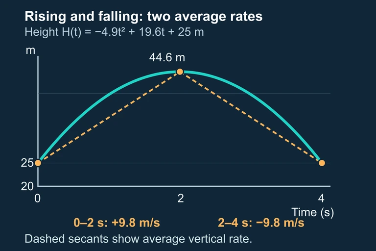 The ball rises from 25 m to 44.6 m and returns to roof height; the two equal-duration average vertical rates have opposite signs. The pictured ball positions form a laterally arranged illustrative sequence, not a measured spatial trajectory; the authoritative plot describes vertical height over time.
Question 5: CRITICAL THINKING
3 ptsShow answer
SUMMARY
Summary & Review
Summary
The average rate of change (AROC) of a function f over an interval [a, b], defined as (f(b) − f(a))/(b − a), provides the slope of the secant line connecting two points on the graph. For a linear function f(x) = mx + b, the AROC equals the slope m for every interval—a constant rate of change that produces a straight-line graph. For a quadratic function f(x) = ax² + bx + c, the AROC = a(x₁ + x₂) + b is a linear function of the endpoints, producing a parabolic graph whose curvature reflects the changing rate of change.
The difference table is the primary diagnostic tool: constant first differences confirm a linear model, while constant second differences (equal to 2ah² for step size h) confirm a quadratic model. The vertex of a quadratic at x = −b/(2a) is the point where the rate of change is zero, and the AROC over any symmetric interval centered at the vertex is zero. These precalculus ideas connect directly to the derivative in calculus, where the AROC becomes the instantaneous rate of change as the interval width approaches zero.