The Inverse and Determinant of a Matrix - AP Precalculus

SECTION 1

Historical Context & Motivation

The study of matrices arose from the practical need to solve systems of linear equations — a problem that appears in virtually every branch of science, engineering, and economics. Long before the formal notion of a matrix existed, mathematicians in China, Persia, and Europe devised systematic elimination methods for solving such systems. The modern matrix concept crystallized in the nineteenth century when Arthur Cayley and James Joseph Sylvester formalized the rules of matrix algebra, including the pivotal ideas of the determinant and the matrix inverse. These two concepts answer a deceptively simple question: given a matrix equation AX = B, can we 'divide' both sides by A to isolate X?

~200 BCE • Chinese Method of Rectangular Arrays

The Nine Chapters on the Mathematical Art describes a tabular elimination method for solving systems of linear equations — an early precursor to Gaussian elimination and matrix representation.

1693 • Leibniz Introduces the Determinant Concept

Gottfried Wilhelm Leibniz recognized that the solvability of a system of linear equations could be captured by a single numerical expression computed from the coefficients — what we now call the determinant.

1750 • Cramer's Rule Published

Gabriel Cramer formalized a method for solving linear systems using ratios of determinants, establishing a direct link between the determinant and the existence of a unique solution.

1858 • Cayley Defines Matrix Algebra

Arthur Cayley published A Memoir on the Theory of Matrices, formally defining matrix multiplication, the identity matrix, and the inverse of a matrix — unifying decades of scattered results into a coherent algebraic framework.

20th c. • Computational Revolution

With the advent of digital computers, efficient algorithms for computing determinants and inverses (LU decomposition, etc.) enabled real-time applications in computer graphics, data science, and machine learning — areas where matrix operations run millions of times per second.

The central question this lesson addresses is: How do we determine whether a square matrix possesses an inverse, and if it does, how do we compute that inverse? The determinant serves as the gatekeeper — a scalar value that tells us whether the inverse exists — while the inverse formula itself provides the algebraic machinery to 'undo' a matrix transformation.

SECTION 2

Core Principles & Definitions

Before computing anything, it is essential to establish the foundational ideas that govern matrix invertibility. In AP Precalculus the focus is on 2 × 2 matrices, which are the simplest non-trivial case and provide a template for understanding larger matrices in later coursework. The four principles below form the conceptual backbone of this topic.

The Identity Matrix I

The identity matrix I is the matrix equivalent of the number 1 in ordinary multiplication: for any square matrix A, AI = IA = A. For 2 × 2 matrices, I = [[1, 0], [0, 1]].

The Determinant det(A)

For A = [[a, b], [c, d]], the determinant is the scalar ad − bc. It measures the signed area-scaling factor of the linear transformation represented by A and determines whether the inverse exists.

Invertibility Criterion

A square matrix A is invertible (also called nonsingular) if and only if det(A) ≠ 0. When det(A) = 0 the matrix is singular and no inverse exists.

The Inverse Matrix A⁻¹

If A is invertible, there exists a unique matrix A⁻¹ such that AA⁻¹ = A⁻¹A = I. The inverse 'undoes' the transformation performed by A, enabling us to solve AX = B as X = A⁻¹B.

✦

KEY TAKEAWAY

Think of a matrix as a machine that transforms input vectors into output vectors. The inverse matrix is the reverse gear of that machine — it takes every output back to its original input. The determinant is the 'diagnostic light' on the dashboard: if it reads zero, the machine has collapsed two or more distinct inputs onto the same output, making the process irreversible. Just as an engineer cannot reverse a lossy compression algorithm, you cannot invert a singular matrix because information has been destroyed.

SECTION 3

Geometric Interpretation of the Determinant

The determinant of a 2 × 2 matrix has a beautiful geometric meaning: it represents the signed area of the parallelogram formed by the column vectors of the matrix. When that area is nonzero, the two column vectors span all of ℝ², and the transformation is reversible. When the area collapses to zero, the columns are parallel (or one is the zero vector), and the transformation crushes the entire plane onto a line or a point — making inversion impossible. The diagram below illustrates these two cases side by side.

Left: The matrix A = [[3, 1], [1, 2]] has det(A) = 5. Its column vectors form a parallelogram with area 5, confirming invertibility. Right: The matrix B = [[2, 6], [1, 3]] has det(B) = 0. The columns are scalar multiples of each other, so the parallelogram collapses to a line segment — no inverse exists.

In the left panel, the cyan vector col₁ = (3, 1) and the violet vector col₂ = (1, 2) point in genuinely different directions, sweeping out a parallelogram whose area equals |det(A)| = 5. Because the transformation spreads input vectors across a two-dimensional region, every output can be traced back to exactly one input — the hallmark of invertibility. In the right panel, col₂ = 3 × col₁, so both columns lie along the same line. The 'parallelogram' has zero width, the determinant equals zero, and the mapping is irreversible.

SECTION 4

Mathematical Framework

For the AP Precalculus course, the formulas you need involve 2 × 2 matrices. Let A be the general 2 × 2 matrix with entries a, b, c, and d arranged as A = [[a, b], [c, d]]. Three key formulas govern the determinant, the inverse, and the solution of a matrix equation.

DETERMINANT OF A 2 × 2 MATRIX

det(A) = ad − bc

where a and d are the entries on the main diagonal (top-left to bottom-right), and b and c are the off-diagonal entries. The product of the main diagonal minus the product of the anti-diagonal yields a single scalar.

INVERSE OF A 2 × 2 MATRIX

A⁻¹ = (1 / det(A)) × [[d, −b], [−c, a]]

To build A⁻¹: (1) swap the main-diagonal entries a and d, (2) negate the off-diagonal entries b and c, and (3) multiply the resulting matrix by the scalar 1/det(A). This formula is valid only when det(A) ≠ 0.

SOLVING A MATRIX EQUATION AX = B

X = A⁻¹ B

Just as dividing both sides of 5x = 15 by 5 gives x = 3, pre-multiplying both sides of AX = B by A⁻¹ yields X = A⁻¹B. Note that order matters: because matrix multiplication is not commutative, A⁻¹ must be applied on the left of both sides.

💡

Why Swap and Negate?

The matrix [[d, −b], [−c, a]] is called the adjugate (or classical adjoint) of A. When you multiply A by its adjugate, the cross-terms cancel perfectly, leaving det(A) × I. Dividing by det(A) then produces the identity, which is precisely what A⁻¹ must achieve. This elegant cancellation is why the 'swap diagonals, negate off-diagonals' recipe works.

SECTION 5

Step-by-Step Inverse Formula Breakdown

Let us break the inverse formula into a visual, step-by-step procedure using a concrete example. Consider the matrix A = [[5, 3], [2, 4]]. The diagram below traces every sub-operation, from computing the determinant through to the final inverse matrix.

The six-step pipeline for computing A⁻¹: start with A, compute the determinant, verify it is nonzero, form the adjugate by swapping and negating, scale by 1/det(A), and verify by multiplying AA⁻¹ to confirm the identity matrix.

Notice that the verification step (Step 6) is not merely a formality — it is a powerful self-check that catches arithmetic errors before they propagate into downstream calculations. On the AP exam, quickly multiplying your candidate inverse by the original matrix is an efficient way to confirm your answer, especially under time pressure.

SECTION 6

Worked Example: Solving a System with A⁻¹

One of the most important applications of the matrix inverse is solving a system of two linear equations in two unknowns. Suppose we need to solve the system 3x + 7y = 1 and 2x + 5y = 3. We can rewrite this system in matrix form as AX = B, where A is the coefficient matrix, X is the variable column, and B is the constant column. Then X = A⁻¹B gives the solution directly.

Solving 3x + 7y = 1, 2x + 5y = 3 Using the Matrix Inverse

1
Step 1 — Write in Matrix Form AX = B

Identify the coefficient matrix A = [[3, 7], [2, 5]], the variable vector X = [[x], [y]], and the constant vector B = [[1], [3]]. The system becomes AX = B.
2
Step 2 — Compute the Determinant

det(A) = (3)(5) − (7)(2) = 15 − 14 = 1.

det(A) = 1 ≠ 0, so A is invertible.
3
Step 3 — Form the Inverse

Apply the formula A⁻¹ = (1/det(A)) × [[d, −b], [−c, a]]. Swap the diagonal entries (3 ↔ 5) and negate the off-diagonal entries (7 → −7, 2 → −2). Since det(A) = 1, the scalar factor is simply 1. Therefore A⁻¹ = [[5, −7], [−2, 3]].

A⁻¹ = [[5, −7], [−2, 3]]
4
Step 4 — Multiply X = A⁻¹B

X = [[5, −7], [−2, 3]] × [[1], [3]]. For the first entry: 5(1) + (−7)(3) = 5 − 21 = −16. For the second entry: (−2)(1) + 3(3) = −2 + 9 = 7.

X = [[−16], [7]], so x = −16 and y = 7.
5
Step 5 — Verify in Original Equations

Equation 1: 3(−16) + 7(7) = −48 + 49 = 1 ✓. Equation 2: 2(−16) + 5(7) = −32 + 35 = 3 ✓. Both equations are satisfied.

Solution confirmed: (x, y) = (−16, 7).

SECTION 7

Matrix Inverse vs. Other Solution Methods

The matrix inverse is not the only tool for solving linear systems. Two common alternatives — substitution/elimination and Cramer's Rule — also appear in precalculus coursework. Each approach has distinct advantages and limitations, summarized below.

Feature	Matrix Inverse (A⁻¹B)	Substitution / Elimination	Cramer's Rule
Best for	Solving multiple systems with the same A but different B vectors	Quick ad-hoc solutions for small systems; no matrix setup needed	Finding one specific variable without solving the full system
Requires	det(A) ≠ 0; matrix algebra knowledge	No prerequisites beyond algebra	det(A) ≠ 0; computation of multiple determinants
Limitation	Only works for square, invertible coefficient matrices	No compact formula; harder to generalize to n × n systems	Computationally expensive for n > 3 due to multiple determinant evaluations
AP Exam relevance	Frequently tested in matrix-form questions and FRQs	Assumed prerequisite skill; rarely the focus of matrix questions	Occasionally tested as an alternative approach

Comparison of three methods for solving 2 × 2 linear systems

🔑

WHEN TO USE WHICH METHOD

If the AP exam presents a system in matrix form and asks you to solve it, the matrix inverse method is almost certainly the expected approach. However, if you only need the value of one variable, Cramer's Rule can be faster. Think of the inverse as a reusable key that opens every door in a building (every B vector), while Cramer's Rule is a single-use lockpick — effective for one door at a time.

SECTION 8

Connection to Higher-Dimensional Matrices & Linear Algebra

The 2 × 2 framework you have learned generalizes naturally to n × n matrices in a college linear algebra course. The determinant still determines invertibility, the inverse still satisfies AA⁻¹ = I, and the solution to AX = B still takes the form X = A⁻¹B. However, the computational methods scale dramatically: for a 3 × 3 matrix the determinant involves six triple-products, and for larger matrices, cofactor expansion or row-reduction algorithms become necessary. The table below previews how key ideas extend.

Concept	2 × 2 (AP Precalculus)	n × n (Linear Algebra)
Determinant	ad − bc (single formula)	Cofactor expansion or row-reduction; produces a scalar
Inverse formula	(1/det) × adjugate (swap & negate)	(1/det) × adj(A); adjugate built from cofactor matrix
Geometric meaning of det	Signed area of parallelogram	Signed volume of parallelotope in ℝⁿ
Practical computation	By-hand formula; calculator for verification	Gaussian elimination or LU decomposition (computer algorithms)

From AP Precalculus to college linear algebra

Understanding the 2 × 2 case deeply — why the determinant governs invertibility, how the adjugate achieves cancellation, and why singular matrices destroy information — gives you a conceptual foundation that transfers directly to higher dimensions. In courses such as multivariable calculus, differential equations, and data science, matrix inverses appear in contexts ranging from Jacobian transformations to least-squares regression, making this one of the most transferable ideas in all of mathematics.

SECTION 9

Practice Problems

Question 1: CONCEPTUAL

If det(A) = 0 for a 2 × 2 matrix A, which of the following statements must be true?

A. A is the zero matrix.
B. The system AX = B has infinitely many solutions for every B.
C. A does not have an inverse.
D. All entries of A are equal.
E. A has exactly one eigenvalue equal to zero.

Show answer (C)

The correct answer is C. A matrix is invertible if and only if its determinant is nonzero; therefore det(A) = 0 means A has no inverse. A is wrong because many non-zero matrices (e.g., [[1, 2], [2, 4]]) have determinant zero. B is wrong because a singular matrix may produce no solutions (inconsistent) or infinitely many solutions depending on B — it is not guaranteed to be infinitely many for every B. D is wrong because having equal entries is a very specific structure unrelated to the general condition det = 0. E is wrong because a 2 × 2 singular matrix could have zero as a repeated eigenvalue (e.g., the zero matrix), so 'exactly one' is not necessarily true.

Question 2: BASIC CALCULATION

What is the inverse of A = [[4, 1], [6, 2]]?

A. [[2, −1], [−6, 4]]
B. [[1, −1/2], [−3, 2]]
C. The inverse does not exist.
D. [[ −2, 1], [6, −4]]
E. [[1/4, −1/6], [−1, 1/2]]

Show answer (B)

The correct answer is B. First compute det(A) = 4(2) − 1(6) = 8 − 6 = 2 ≠ 0, so the inverse exists (ruling out C). The adjugate is [[2, −1], [−6, 4]], and scaling by 1/det = 1/2 gives A⁻¹ = [[1, −1/2], [−3, 2]]. A is wrong because it is the adjugate without the 1/det scaling. D is wrong because it negates the diagonal entries incorrectly (they should be swapped, not negated). E is wrong because it takes reciprocals of individual entries, which is not how matrix inversion works.

Question 3: INTERMEDIATE

A 2 × 2 matrix A satisfies det(A) = −3. What is det(A⁻¹)?

A. 3
B. −3
C. −1/3
D. 1/3
E. 9

Show answer (C)

The correct answer is C. Since AA⁻¹ = I, taking determinants of both sides yields det(A) × det(A⁻¹) = det(I) = 1. Therefore det(A⁻¹) = 1/det(A) = 1/(−3) = −1/3. A is wrong because it takes |det(A)| rather than the reciprocal. B is wrong because det(A⁻¹) is the reciprocal of det(A), not det(A) itself. D is wrong because it takes the absolute value of the reciprocal, losing the negative sign. E is wrong because it squares the determinant rather than taking its reciprocal.

Question 4: APPLIED

4 pts

A nutritionist mixes two supplements, X and Y. Each serving of X provides 5 mg of iron and 3 mg of zinc. Each serving of Y provides 2 mg of iron and 4 mg of zinc. A patient needs exactly 16 mg of iron and 18 mg of zinc per day. (a) Write the system as a matrix equation AX = B, identifying A, X, and B. (b) Compute det(A) and determine whether A is invertible. (c) Find A⁻¹. (d) Use A⁻¹ to solve for the number of servings of each supplement.

Show answer

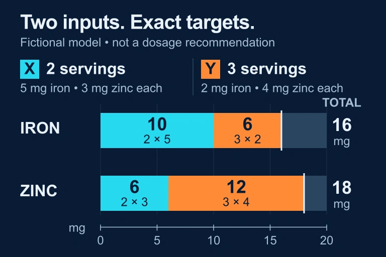
Point 1 (1 pt) — Setting up the matrix equation: Let x = servings of X and y = servings of Y. The system is 5x + 2y = 16 and 3x + 4y = 18. In matrix form: A = [[5, 2], [3, 4]], X = [[x], [y]], B = [[16], [18]], so AX = B. Point 2 (1 pt) — Computing the determinant: det(A) = 5(4) − 2(3) = 20 − 6 = 14. Since 14 ≠ 0, A is invertible. Point 3 (1 pt) — Finding A⁻¹: The adjugate is [[4, −2], [−3, 5]]. Scaling by 1/14: A⁻¹ = (1/14)[[4, −2], [−3, 5]] = [[2/7, −1/7], [−3/14, 5/14]]. Point 4 (1 pt) — Solving for X: X = A⁻¹B = (1/14)[[4, −2], [−3, 5]] × [[16], [18]] = (1/14)[[4(16) + (−2)(18)], [(−3)(16) + 5(18)]] = (1/14)[[64 − 36], [−48 + 90]] = (1/14)[[28], [42]] = [[2], [3]]. The patient needs 2 servings of X and 3 servings of Y per day. Verification: 5(2) + 2(3) = 16 ✓ and 3(2) + 4(3) = 18 ✓. Two servings of X and three of Y give iron contributions 10+6=16 mg and zinc contributions 6+12=18 mg in stacked bars.

Two servings of X and three of Y give iron contributions 10+6=16 mg and zinc contributions 6+12=18 mg in stacked bars.

Question 5: CRITICAL THINKING

3 pts

Let A = [[k, 4], [2, k]] where k is a real number. (a) For what values of k is A singular? (b) For a value of k that makes A invertible, show that det(A) × det(A⁻¹) = 1. (c) Explain geometrically what happens to the column vectors of A as k approaches one of the singular values you found in part (a).

Show answer

Point 1 (1 pt) — Finding singular values: A is singular when det(A) = 0. det(A) = k² − 8. Setting k² − 8 = 0 gives k² = 8, so k = 2√2 or k = −2√2. These are the two values of k for which A has no inverse. Point 2 (1 pt) — Verifying the determinant reciprocal property: Choose k = 3 (which gives det(A) = 9 − 8 = 1). Then A = [[3, 4], [2, 3]] and A⁻¹ = [[3, −4], [−2, 3]]. det(A⁻¹) = 3(3) − (−4)(−2) = 9 − 8 = 1. Thus det(A) × det(A⁻¹) = 1 × 1 = 1. More generally, for any invertible k: since AA⁻¹ = I, det(A) × det(A⁻¹) = det(I) = 1, by the multiplicative property of determinants. Point 3 (1 pt) — Geometric explanation: The columns of A are (k, 2) and (4, k). As k → 2√2, the column vectors approach (2√2, 2) and (4, 2√2). Note that (4, 2√2) = √2 × (2√2, 2), so the second column becomes a scalar multiple of the first. Geometrically, the parallelogram formed by the two column vectors 'flattens' as the vectors become parallel, and its area (|det(A)| = |k² − 8|) shrinks to zero. At the singular value, both columns point in the same direction and the transformation collapses ℝ² onto a single line, making inversion impossible.

SUMMARY

Lesson Summary

Summary

The determinant of a 2 × 2 matrix A = [[a, b], [c, d]] is the scalar ad − bc, which measures the signed area-scaling factor of the linear transformation. A matrix is invertible if and only if its determinant is nonzero; when the determinant equals zero, the matrix is singular and no inverse exists because the transformation collapses the plane, destroying information.

When the inverse exists, the formula A⁻¹ = (1/det(A)) × [[d, −b], [−c, a]] provides it directly — swap the main-diagonal entries, negate the off-diagonal entries, and scale by the reciprocal of the determinant. The inverse enables the powerful solution strategy X = A⁻¹B for any matrix equation AX = B. Always verify your answer by confirming that AA⁻¹ = I, the identity matrix. Mastering these ideas prepares you not only for the AP Precalculus exam but for the broader landscape of linear algebra that underpins modern science and engineering.