Implicitly Defined Functions - AP Precalculus

SECTION 1

Historical Context & Motivation

For most of your mathematical career, functions have appeared in a familiar form: y = f(x), where the dependent variable is neatly isolated on one side of the equation. Yet many of the most important curves in mathematics — circles, ellipses, and higher-order algebraic curves — resist this tidy packaging. The equation x² + y² = 1 defines the unit circle, but no single function y = f(x) captures the entire circle at once. This tension between the richness of geometric curves and the limitations of explicit function notation has driven mathematicians for centuries to develop a more flexible framework: implicit definition.

~300 BCE • Apollonius and the Conic Sections

Apollonius of Perga systematically studied ellipses, parabolas, and hyperbolas — curves that are naturally described by implicit equations relating two variables simultaneously.

1637 • Descartes' Coordinate Geometry

René Descartes introduced the coordinate plane, enabling algebraic equations to represent geometric curves. Equations like x² + y² = r² became central tools, even though they could not be written as a single explicit function.

1736 • Euler's Analytic Methods

Leonhard Euler formalized the distinction between explicit and implicit representations of functions and began exploring how to extract local functional behavior from implicit relations using algebraic manipulation.

1800s • Implicit Function Theorem

Augustin-Louis Cauchy and later mathematicians rigorously proved conditions under which an implicit equation F(x, y) = 0 guarantees the existence of a locally explicit function y = g(x), laying the foundation for modern analysis.

The central question that implicit functions address is deceptively simple: when an equation involves both x and y in an entangled way, can we still treat y as depending on x? In AP Precalculus, understanding implicit definition equips you to work with parametric equations, conic sections, and other relations that transcend the standard y = f(x) framework, connecting naturally to the study of parameters, vectors, and matrices.

SECTION 2

Core Principles & Definitions

An implicitly defined function arises when a relationship between x and y is given by an equation of the form F(x, y) = 0 rather than being solved explicitly for one variable. The equation does not hand you y on a silver platter; instead, it constrains x and y simultaneously, and the functional relationship must be inferred from the structure of the equation. Understanding when and how implicit equations define functions locally — even when they fail to do so globally — is one of the most important conceptual leaps in precalculus.

Explicit vs. Implicit Form

An explicit function directly gives y = f(x). An implicit equation expresses a relationship F(x, y) = 0 without isolating y. For example, y = √(1 − x²) is explicit, while x² + y² = 1 is implicit.

Local vs. Global Function Behavior

An implicit equation may fail the vertical line test globally (like a circle), yet still define y as a function of x in a sufficiently small neighborhood of a point. This local behavior is key to extracting functional information.

Parametric Connection

Many implicitly defined curves can be described parametrically: x = f(t), y = g(t). Parameters provide a way to trace the curve point-by-point, sidestepping the difficulty of solving for y explicitly.

The Role of Constraints

An implicit equation acts as a constraint that reduces the two-dimensional freedom of the (x, y)-plane to a one-dimensional curve. Every point on that curve satisfies the equation, and the curve encodes the functional dependence.

✦

KEY TAKEAWAY

Think of an implicit equation as a contract between x and y: neither variable is "in charge," but both must satisfy the same agreement. It is analogous to a system of GPS satellites constraining your position — the satellites don't tell you your coordinates directly, but the constraint equations among signal arrival times implicitly determine where you are. Similarly, F(x, y) = 0 constrains the pair (x, y) to lie on a specific curve, and near most points on that curve, y is effectively a function of x.

SECTION 3

Visual Explanation

Explicit vs. Implicit: Seeing the Difference

The diagram below contrasts an explicitly defined function with an implicitly defined curve. On the left, the parabola y = x² passes the vertical line test everywhere — every x-value maps to exactly one y-value. On the right, the unit circle x² + y² = 1 fails the vertical line test globally, since most x-values in (−1, 1) correspond to two y-values. Yet if we restrict attention to just the upper semicircle (shown in cyan), we recover a genuine function y = √(1 − x²). This illustrates the fundamental idea that implicit equations can define functions locally even when they do not do so globally.

Left: The parabola y = x² passes the vertical line test — every vertical line (gold, dashed) hits the curve at most once. Right: The full circle (pink, dashed) fails the vertical line test, but the upper semicircle (cyan, solid) defines y as a function of x locally.

Notice the gold vertical line on the right side of the diagram intersects the full circle at two points — one on the upper semicircle and one on the lower semicircle. This is precisely why the full circle is a relation rather than a function. However, if you restrict your view to just the upper arc (or just the lower arc), each vertical line intersects the curve at exactly one point, and you recover a bona fide function. This restriction process is at the heart of extracting explicit functions from implicit equations.

SECTION 4

Mathematical Framework

Working with implicitly defined functions requires a mathematical toolkit for determining when a function exists, how to find points on the curve, and how to convert between implicit, explicit, and parametric representations. Below we formalize the key equations and procedures you will encounter in AP Precalculus.

GENERAL IMPLICIT EQUATION

F(x, y) = 0

F is an expression involving both x and y. A point (a, b) lies on the curve if and only if F(a, b) = 0. The set of all such points forms the solution set or level curve of F at 0.

CIRCLE (STANDARD FORM)

(x − h)² + (y − k)² = r²

Center (h, k), radius r. This is implicitly defined because expanding and rearranging gives F(x, y) = (x − h)² + (y − k)² − r² = 0. Solving for y yields two branches: y = k ± √(r² − (x − h)²).

ELLIPSE (STANDARD FORM)

x²/a² + y²/b² = 1

Semi-major axis a along the x-axis, semi-minor axis b along the y-axis (when a > b). Solving for y gives two branches: y = ±b√(1 − x²/a²). The implicit form naturally arises when modeling orbits, optics, and engineering cross-sections.

PARAMETRIC CONVERSION

x = r cos(t), y = r sin(t), 0 ≤ t < 2π

The unit circle x² + y² = r² can be re-expressed parametrically. The parameter t sweeps through all angles, and each value of t produces a unique point on the circle. This conversion transforms the implicit constraint into a pair of explicit equations in terms of the parameter t.

💡

When Can You Solve for y?

At the AP Precalculus level, you will primarily encounter implicit equations that are polynomial in y. If the equation is linear in y (e.g., 3x²y + 2x = 7 can be solved as y = (7 − 2x)/(3x²)), you can always isolate y. If the equation is quadratic in y, the quadratic formula yields two branches. Higher-degree or transcendental implicit equations (like x sin(y) = y cos(x)) typically cannot be solved algebraically and require numerical or graphical methods.

SECTION 5

Types & Classification of Implicit Curves

Implicitly defined curves come in a rich variety of forms, and classifying them helps you predict their behavior, the number of explicit branches, and the best strategy for analysis. The diagram below organizes the most important families of implicit curves you will encounter, along with their parametric counterparts and the number of explicit branches that arise when solving for y.

A classification of common implicitly defined curves. Conic sections (circle, ellipse, hyperbola) produce two explicit branches when solved for y. Equations linear in y always yield a single branch. Higher-order curves like the Folium of Descartes may require parametric representation because closed-form solutions for y do not exist.

Curve Type	Implicit Form	# of y-Branches	Parametric Available?
Circle	x² + y² = r²	2	Yes: x = r cos t, y = r sin t
Ellipse	x²/a² + y²/b² = 1	2	Yes: x = a cos t, y = b sin t
Hyperbola	x²/a² − y²/b² = 1	2	Yes: x = a sec t, y = b tan t
Line (implicit)	Ax + By + C = 0	1	Yes: x = t, y = (−At − C)/B
Folium of Descartes	x³ + y³ = 3axy	No closed form	Yes: rational parametrization in t

Summary of common implicit curves and their properties

SECTION 6

Worked Example

Let us work through a complete example that showcases the process of analyzing an implicitly defined function: determining points on the curve, solving for explicit branches, and converting to parametric form.

Analyzing the Ellipse 4x² + 9y² = 36

1
Step 1 — Rewrite in Standard Form

Divide every term by 36 to obtain x²/9 + y²/4 = 1. This reveals the equation is an ellipse centered at the origin with a² = 9 and b² = 4.

x²/9 + y²/4 = 1, so a = 3, b = 2
2
Step 2 — Verify a Specific Point

Check whether the point (3, 0) lies on the curve by substituting: 4(3)² + 9(0)² = 4(9) + 0 = 36. Since 36 = 36, the point satisfies the equation. Similarly, (0, 2) gives 4(0)² + 9(2)² = 9(4) = 36 ✓.

(3, 0) and (0, 2) lie on the ellipse
3
Step 3 — Solve for y Explicitly

Starting from 4x² + 9y² = 36, isolate y²: 9y² = 36 − 4x², so y² = (36 − 4x²)/9 = 4(9 − x²)/9. Taking the square root of both sides yields two branches: y = +(2/3)√(9 − x²) for the upper half and y = −(2/3)√(9 − x²) for the lower half. The domain restriction is 9 − x² ≥ 0, which gives −3 ≤ x ≤ 3.

y = ±(2/3)√(9 − x²), domain: [−3, 3]
4
Step 4 — Convert to Parametric Form

Using the standard parametric equations for an ellipse with semi-major axis a = 3 and semi-minor axis b = 2, we write x = 3 cos(t) and y = 2 sin(t) for 0 ≤ t < 2π. To verify, substitute: (3 cos t)²/9 + (2 sin t)²/4 = cos²t + sin²t = 1 ✓. Each value of t traces a unique point on the ellipse, and the parameter t can be interpreted as the eccentric anomaly angle.

x = 3 cos(t), y = 2 sin(t), 0 ≤ t < 2π
5
Step 5 — Identify Where Each Branch Is a Function

The upper branch y = (2/3)√(9 − x²) is a function on [−3, 3] since the positive square root is single-valued. The lower branch y = −(2/3)√(9 − x²) is likewise a function on the same domain. Neither branch alone captures the full ellipse, but together they reconstruct the entire implicit curve. At the endpoints x = ±3, the two branches meet (y = 0), confirming that the ellipse is a single connected curve.

Each branch is a function on [−3, 3]; they meet at (±3, 0)

SECTION 7

Explicit, Implicit, and Parametric: Strengths & Limitations

Choosing the right representation for a curve — explicit, implicit, or parametric — depends on the context and what you need to accomplish. Each form has distinct advantages and trade-offs. The table below provides a systematic comparison, highlighting when each representation shines and where it falls short.

Feature	Explicit y = f(x)	Implicit F(x, y) = 0	Parametric x = f(t), y = g(t)
Ease of graphing	Straightforward: plug in x, get y	Harder: test points or use technology	Moderate: compute (x, y) for each t
Multi-valued curves	Cannot handle (fails VLT)	Handles naturally	Handles naturally
Finding slope (dy/dx)	Direct differentiation	Implicit differentiation required	(dy/dt) / (dx/dt)
Direction / motion	No inherent direction	No inherent direction	Yes: t provides orientation
Best suited for	Standard functions, quick evaluation	Conics, algebraic curves, constraints	Motion, animation, tracing curves

Comparison of explicit, implicit, and parametric representations

✦

KEY TAKEAWAY

Think of the three representations as different languages for describing the same geometric object — like architectural blueprints versus a 3D model versus a step-by-step construction manual. The implicit form is the blueprint: it tells you what relationship must hold. The explicit form is the 3D model: you can directly read off outputs. The parametric form is the construction manual: it walks you through the curve point by point. Fluency in translating among all three is the hallmark of precalculus mastery.

SECTION 8

Connection to Calculus & Advanced Theory

Implicitly defined functions form a bridge between precalculus and the powerful techniques of calculus and multivariable analysis. In AP Calculus, you will encounter implicit differentiation, a procedure for finding dy/dx directly from F(x, y) = 0 without first solving for y. The Implicit Function Theorem in advanced mathematics provides rigorous conditions under which a smooth implicit equation guarantees a locally smooth explicit function — conditions that rely on partial derivatives, a concept from multivariable calculus.

Concept	AP Precalculus Level	Calculus / Advanced Level
Defining a function from F(x,y) = 0	Solve algebraically for y; identify branches and domain restrictions	Apply the Implicit Function Theorem using partial derivatives ∂F/∂y ≠ 0
Finding slope	Differentiate the explicit branch y = g(x)	Implicit differentiation: dy/dx = −(∂F/∂x)/(∂F/∂y)
Parametric curves	Convert between implicit and parametric forms for conics	General parametrizations; arc length, curvature, vector-valued functions
Multiple variables	Two variables x and y constrained by one equation	Surfaces F(x, y, z) = 0 in 3D; level surfaces, gradients, tangent planes

Progression from precalculus to advanced treatment of implicit functions

For now, the most important skill is recognizing when an equation implicitly defines a function, extracting explicit branches when possible, and fluently converting to parametric form. These competencies form the scaffolding upon which implicit differentiation, related rates problems, and vector analysis are built in subsequent courses. Mastering the precalculus perspective ensures that when you encounter dy/dx = −(∂F/∂x)/(∂F/∂y) in calculus, the underlying geometric intuition is already in place.

SECTION 9

Practice Problems

Question 1: CONCEPTUAL

Which of the following best explains why the equation x² + y² = 25 does not define y as a function of x over its entire domain?

A. The equation has no real solutions for y when x > 5.
B. For most x-values in (−5, 5), there are two y-values satisfying the equation, so it fails the vertical line test.
C. The equation is not a polynomial, so it cannot define a function.
D. The domain of x is the empty set since x² + y² can never equal 25.
E. The equation defines y as a function of x because circles are standard mathematical functions.

Show answer (B)

Correct Answer: B. For a given x in (−5, 5), solving x² + y² = 25 for y yields y = ±√(25 − x²), producing two outputs for each input — a direct violation of the vertical line test. Choice A is incorrect because solutions do exist for |x| < 5 (and the issue isn't about x > 5 specifically). Choice C is wrong because x² + y² = 25 is indeed a polynomial equation in x and y, and polynomials certainly can define functions. Choice D is absurd; for example, (3, 4) satisfies the equation. Choice E is incorrect because the full circle is a relation, not a function.

Question 2: BASIC CALCULATION

Given the implicit equation 9x² + 4y² = 36, which of the following represents the upper branch of the curve solved explicitly for y?

A. y = (3/2)√(4 + x²)
B. y = (2/3)√(9 − x²)
C. y = (3/2)√(4 − x²)
D. y = (3/2)√(4 − x²/9)
E. y = 3√(1 − x²)

Show answer (C)

Correct Answer: C. Starting from 9x² + 4y² = 36, divide both sides by 36 to obtain the standard form: x²/4 + y²/9 = 1. This is an ellipse with semi-axis a = 2 along x and semi-axis b = 3 along y. Isolating y²: y² = 9(1 − x²/4) = (9/4)(4 − x²). Taking the positive square root for the upper branch: y = (3/2)√(4 − x²). Verify at x = 0: y = (3/2)√4 = (3/2)(2) = 3. Check: 9(0) + 4(9) = 36 ✓. Verify at x = 2: y = (3/2)√(4 − 4) = 0. Check: 9(4) + 4(0) = 36 ✓. Now check the wrong answers. Choice A: y = (3/2)√(4 + x²) is increasing for x > 0 and gives y = (3/2)(2) = 3 at x = 0, but at x = 2: y = (3/2)√8 = 3√2 ≈ 4.24, and 9(4) + 4(18) = 36 + 72 = 108 ≠ 36 ✗. Also, this expression is not bounded, unlike an ellipse. Choice B: y = (2/3)√(9 − x²) gives y = (2/3)(3) = 2 at x = 0, and 9(0) + 4(4) = 16 ≠ 36 ✗. Choice D: y = (3/2)√(4 − x²/9) gives y = (3/2)(2) = 3 at x = 0 ✓, but at x = 3: y = (3/2)√(4 − 1) = (3/2)√3 ≈ 2.60, and 9(9) + 4(6.75) = 81 + 27 = 108 ≠ 36 ✗. Choice E: y = 3√(1 − x²) gives y = 3 at x = 0 ✓, but the domain is only |x| ≤ 1, while the ellipse extends to |x| ≤ 2. At x = 1: y = 3√0 = 0, and 9(1) + 4(0) = 9 ≠ 36 ✗. Only choice C is correct.

Question 3: INTERMEDIATE

3 pts

Consider the implicit equation xy + 2y = x² − 1. Solve for y as an explicit function of x, and state the domain of the resulting function.

Show answer

Point 1 (1 pt) — Factor and isolate y: Rewrite the equation as y(x + 2) = x² − 1. Factor the right side: x² − 1 = (x − 1)(x + 1). Therefore y = (x − 1)(x + 1)/(x + 2). Point 2 (1 pt) — State the explicit function: y = (x² − 1)/(x + 2). This is a single branch since the original equation is linear in y, confirming it defines y as a function of x (not a multi-valued relation). Point 3 (1 pt) — Determine the domain: The denominator x + 2 = 0 when x = −2, so the domain is all real numbers except x = −2, written as (−∞, −2) ∪ (−2, ∞). At x = −2, the implicit equation has no solution for y because 0 · y = (−2)² − 1 = 3 yields the contradiction 0 = 3.

Question 4: APPLIED

5 pts

An engineer models the cross-section of an elliptical tunnel using the implicit equation x²/16 + y²/9 = 1, where x and y are measured in meters and y ≥ 0 represents the height above ground level. (a) Write the parametric equations for the full ellipse. (b) Determine the explicit function y = f(x) for the tunnel's upper profile and state its domain. (c) A vehicle that is 2.5 meters tall needs to pass through the tunnel. Find the maximum width of a lane centered at x = 0 such that the vehicle can pass. Justify your answer with calculations. (d) Explain why the implicit equation, rather than the explicit form alone, is valuable for an engineer designing this tunnel.

Show answer

Point 1 (1 pt) — Parametric equations: With a = 4 and b = 3, the parametric form is x = 4 cos(t), y = 3 sin(t), for 0 ≤ t < 2π. For just the upper half (tunnel profile), restrict to 0 ≤ t ≤ π. Point 2 (1 pt) — Explicit upper branch: From x²/16 + y²/9 = 1, solve: y² = 9(1 − x²/16) = 9(16 − x²)/16. Since y ≥ 0, y = (3/4)√(16 − x²). The domain is −4 ≤ x ≤ 4, since 16 − x² ≥ 0 requires |x| ≤ 4. Point 3 (2 pts) — Maximum lane width: The vehicle has height 2.5 m. Set y = 2.5 and solve for x: 2.5 = (3/4)√(16 − x²) → 10/3 = √(16 − x²) → 100/9 = 16 − x² → x² = 16 − 100/9 = 144/9 − 100/9 = 44/9 → x = ±√(44/9) = ±(2√11)/3 ≈ ±2.211 m. The maximum width of a centered lane is 2 × (2√11)/3 = (4√11)/3 ≈ 4.42 meters. At any horizontal distance from center less than about 2.21 m, the tunnel height exceeds 2.5 m, so the vehicle can pass. Point 4 (1 pt) — Why implicit form is valuable: The implicit equation x²/16 + y²/9 = 1 describes the entire cross-section in a single compact expression, making it easy to check whether any point (x, y) lies inside, on, or outside the tunnel boundary. This is critical for engineering design: verifying clearance involves substituting coordinates directly into F(x, y) = x²/16 + y²/9 − 1 and checking whether the result is ≤ 0. The explicit form only provides the upper half and requires choosing the correct branch, which is more cumbersome for full boundary analysis. Upper ellipse with a centered inscribed rectangle of height 2.5 and width 4√11/3. The top corners lie on the ellipse.

Upper ellipse with a centered inscribed rectangle of height 2.5 and width 4√11/3. The top corners lie on the ellipse.

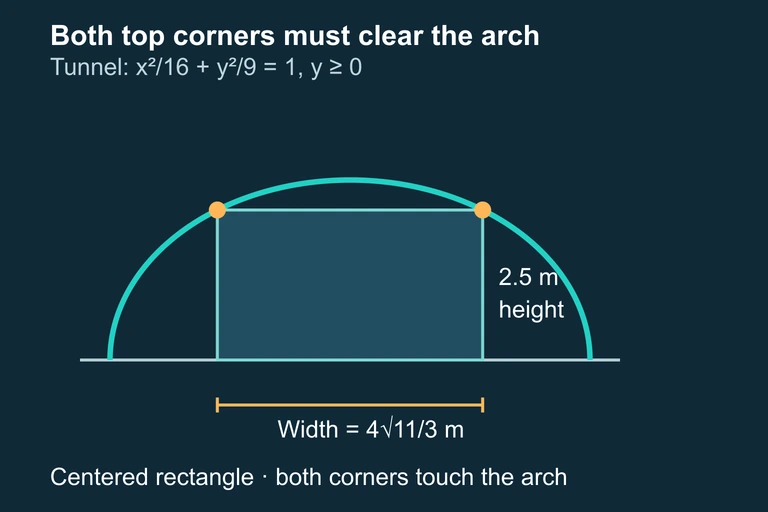Both upper vehicle corners must fit beneath the elliptical arch; at 2.5 m height the maximum centered width is 4√11/3 m.

Question 5: CRITICAL THINKING

Consider the equation x² + xy + y² = 7. (a) Verify that the point (1, 2) lies on the curve. (b) Treating this as a quadratic equation in y, use the quadratic formula to express y explicitly in terms of x. (c) Determine which branch contains the point (1, 2), and state the domain of that branch. (d) Explain why there exist exactly two branches and identify the x-values where the two branches meet.

A. The branches are y = (−x ± √(28 − 3x²))/2; they meet at x = ±2√(7/3); (1, 2) is on the + branch.
B. The branches are y = (−x ± √(28 + 3x²))/2; they meet only at x = 0; (1, 2) is on the + branch.
C. The branches are y = (x ± √(28 − 3x²))/2; they meet at x = ±2√(7/3); (1, 2) is on the − branch.
D. The branches are y = (−x ± √(28 − 3x²))/2; they meet at x = ±√7; (1, 2) is on the − branch.
E. The equation cannot be solved for y using the quadratic formula because the discriminant is always negative.

Show answer (A)

Correct Answer: A. First, verify (1, 2): 1² + (1)(2) + 2² = 1 + 2 + 4 = 7 ✓. Treating the equation as a quadratic in y: y² + xy + (x² − 7) = 0. By the quadratic formula with a = 1, b = x, c = x² − 7: y = (−x ± √(x² − 4(x² − 7)))/2 = (−x ± √(28 − 3x²))/2. This confirms the form in choices A and D. The discriminant 28 − 3x² ≥ 0 requires x² ≤ 28/3, i.e., |x| ≤ 2√(7/3) ≈ 3.055. The two branches meet where the discriminant equals zero: 28 − 3x² = 0, giving x = ±2√(7/3). Now check which branch contains (1, 2): y = (−1 + √(28 − 3))/2 = (−1 + √25)/2 = (−1 + 5)/2 = 4/2 = 2 ✓, so (1, 2) lies on the + branch. Choice B is wrong because the discriminant is 28 − 3x² (minus, not plus), and the branches do not meet only at x = 0. Choice C incorrectly writes (x ± ...) instead of (−x ± ...) and misidentifies the branch. Choice D has the correct formula but states the branches meet at x = ±√7 (which would mean 28 − 3·7 = 7 ≠ 0), and misidentifies the branch as −. Choice E is false since the discriminant is non-negative for |x| ≤ 2√(7/3).

SUMMARY

Lesson Summary

Summary

An implicitly defined function arises from an equation F(x, y) = 0 that relates two variables without isolating one as an explicit output. While such equations may fail the vertical line test globally — as with circles, ellipses, and hyperbolas — they can often be decomposed into explicit branches that each define y as a function of x on a restricted domain. The key algebraic technique is to treat the equation as a polynomial in y, use the quadratic formula or direct isolation when possible, and identify the resulting domain restrictions.

When explicit solutions are impractical, parametric equations offer an alternative route: expressing x and y each as functions of a third variable t (the parameter) allows you to trace the entire curve point by point. Fluency in converting among implicit, explicit, and parametric forms is essential for AP Precalculus and forms the bridge to implicit differentiation and vector-valued functions studied in calculus.