Function Model Selection and Assumption Articulation - AP Precalculus

SECTION 1

Historical Context & Motivation

The act of choosing a mathematical function to describe observed phenomena is as old as quantitative science itself. Long before graphing calculators or regression software existed, mathematicians and natural philosophers confronted a fundamental question: given a set of observations, which algebraic form best captures the underlying relationship? This question drives function model selection—the deliberate process of matching data behavior to a function family—and it demands that the modeler explicitly state every assumption that justifies the choice. Without such assumption articulation, a model's predictive power cannot be evaluated, and its domain of validity remains unknown.

~300 BCE • Euclid's Proportional Reasoning

Euclid formalized proportional relationships in Elements, establishing linear and quadratic models as tools for describing geometric quantities and laying the groundwork for algebraic modeling.

1615 • Kepler's Polynomial Interpolation

Johannes Kepler used polynomial relationships to describe planetary motion, selecting power-law models and explicitly noting the assumptions of elliptical orbits—an early instance of model selection grounded in physical reasoning.

1805 • Legendre's Least Squares Method

Adrien-Marie Legendre published the method of least squares, providing a systematic criterion for fitting candidate function models to data and comparing their quality of fit.

1974 • Akaike Information Criterion

Hirotugu Akaike introduced AIC, a formal framework for balancing model fit against complexity—formalizing the idea that a good model is not merely accurate but parsimonious in its assumptions.

The central gap that this lesson addresses is the space between recognizing data patterns and rigorously defending a modeling choice. On the AP Precalculus exam, you are expected not merely to identify whether data looks linear, quadratic, or rational, but to articulate why a particular function family is appropriate, what assumptions are embedded in that choice, and under what conditions the model may break down. This synthesis of quantitative reasoning and verbal justification is the hallmark of mathematical maturity.

SECTION 2

Core Principles & Definitions

Function model selection rests on several interconnected principles that guide the modeler from raw data to a justified algebraic representation. Understanding these principles transforms model selection from guesswork into a disciplined analytical process. Each principle carries embedded assumptions that must be made explicit whenever a model is proposed or defended.

End Behavior & Dominance

As x → ±∞, the dominant term of a polynomial or the ratio of leading terms in a rational function determines long-run behavior. This is the first filter for distinguishing polynomial from rational models: does the output grow without bound, level off, or approach an asymptote?

Rate of Change Patterns

Constant first differences suggest a linear model; constant second differences suggest a quadratic model. For polynomial models of degree n, constant nth differences are the signature. Rational functions exhibit rates of change that themselves involve rational expressions.

Zeros, Poles, and Discontinuities

The locations where a function equals zero (x-intercepts) or is undefined (vertical asymptotes and holes) provide structural fingerprints. Polynomial functions are continuous everywhere; rational functions may have vertical asymptotes where the denominator vanishes.

Concavity and Inflection

The direction and changes of curvature help distinguish among polynomial degrees. A quadratic has one concavity; a cubic has an inflection point. Rational functions can exhibit multiple shifts in concavity near vertical asymptotes.

Parsimony (Simplicity)

When two models fit data equally well, the simpler model—the one with fewer parameters and weaker assumptions—is preferred. A linear model should not be replaced by a cubic unless the data clearly demand additional flexibility.

✦

KEY TAKEAWAY

Think of model selection like choosing a vehicle for a trip. A bicycle (linear model) is perfect for a flat, short commute—few assumptions and easy to operate. A car (quadratic or cubic) handles hills and longer distances but requires fuel and maintenance assumptions. A helicopter (high-degree polynomial or rational function) can navigate any terrain but demands far more assumptions about operating conditions. The best choice depends on the landscape of your data, and you must always state why that vehicle is appropriate.

SECTION 3

Visual Explanation — Comparing Function Families

The diagram below places four major function families on the same coordinate axes so that their contrasting behaviors become visually immediate. When selecting a model, ask yourself which curve's qualitative shape most closely mirrors the data's overall trajectory, paying particular attention to end behavior, symmetry, and the presence or absence of asymptotes.

The blue line (linear) grows at a constant rate. The violet parabola (quadratic) has a single extremum and symmetric end behavior. The pink cubic shows opposite end behaviors and an inflection point. The amber rational function features a vertical asymptote (VA) and a horizontal asymptote (HA), distinguishing it structurally from all polynomial models.

Notice how each function family carries distinct structural signatures. A linear model assumes a constant rate of change—an assumption that must be verified by inspecting first differences or a scatter plot. A quadratic model assumes a single turning point and that both ends of the graph point in the same direction, implying constant second differences. Selecting a cubic or higher-degree polynomial assumes additional turning points and an inflection structure that the data must support. Finally, choosing a rational model assumes the existence of input values where the function is undefined—a qualitative feature absent from all polynomial models. Articulating these assumptions is what transforms a curve-fitting exercise into genuine mathematical modeling.

SECTION 4

Mathematical Framework

The mathematical backbone of model selection involves analyzing the algebraic structure of candidate function families and matching their properties to observed data. Below are the key forms and the diagnostic tests associated with each. In every case, the assumptions required by each model type are stated alongside the formula.

POLYNOMIAL OF DEGREE n

f(x) = aₙxⁿ + aₙ₋₁xⁿ⁻¹ + … + a₁x + a₀

where aₙ ≠ 0. Assumptions: The function is continuous for all real x, has at most n − 1 turning points, and the nth finite differences of equally spaced data are constant.

RATIONAL FUNCTION

r(x) = p(x) / q(x), where p and q are polynomials with q(x) ≠ 0

The degree of p is m and the degree of q is n. Assumptions: There exist values of x where the output is undefined (vertical asymptotes or holes). If m < n, HA at y = 0. If m = n, HA at y = aₘ/bₙ. If m > n, no horizontal asymptote (slant or polynomial end behavior).

FINITE DIFFERENCE TEST (DEGREE n)

Δⁿf = f(x + nh) − C(n,1)·f(x + (n−1)h) + … + (−1)ⁿ·f(x) = constant

For equally spaced inputs with step size h, the nth forward differences of a polynomial of degree n are constant. If Δ¹ values are constant → linear. If Δ² values are constant → quadratic. This test assumes equally spaced inputs—a critical assumption often overlooked on exams.

HORIZONTAL ASYMPTOTE CRITERION

lim(x→±∞) r(x) = lim(x→±∞) [aₘxᵐ / bₙxⁿ]

When selecting a rational model, the end behavior is determined by comparing the degrees m (numerator) and n (denominator). This limit analysis assumes that the data eventually stabilizes toward a long-run value, which must be supported by the context of the problem.

💡

AP Exam Tip

Free-response questions frequently ask you to "justify your choice of model." A complete justification includes: (1) naming the function family, (2) citing specific data features (e.g., constant second differences, presence of an asymptote), and (3) stating the underlying assumption (e.g., "this model assumes the rate of change is proportional to the input"). Merely stating "it looks quadratic" earns minimal credit.

SECTION 5

Model Selection Decision Framework

The following decision diagram provides a systematic workflow for choosing among polynomial and rational function models. Rather than relying on visual intuition alone, this framework uses a sequence of diagnostic questions—each tied to a specific mathematical assumption—to narrow the field of candidate models. Work from the top down, and at each decision node, verify the corresponding assumption against your data.

Begin at the top. The first branch separates rational models (undefined outputs exist) from polynomial models (continuous everywhere). The polynomial branch uses the finite difference test to determine the degree. Each decision node corresponds to a testable assumption that should be articulated in your written justification.

When using this flowchart on an exam, remember that the finite difference test carries a built-in assumption: the input values must be equally spaced. If the x-values in your table are not equally spaced, you must either re-interpolate or rely on other diagnostic criteria such as the number of turning points, the presence of inflection points, or the scatter plot's qualitative shape. Additionally, in applied problems, contextual clues—such as a population that cannot exceed a carrying capacity—may directly suggest a rational model whose horizontal asymptote represents the limit, even before any numerical test is performed.

SECTION 6

Worked Example — Selecting and Justifying a Model

A biologist records the concentration of a nutrient (mg/L) in a lake at equally spaced weekly intervals. The data are shown below. Determine an appropriate function model and articulate the assumptions that support your choice.

Week (t)	Concentration C(t)
0	2.0
1	5.0
2	8.0
3	9.5
4	10.0
5	10.3
6	10.4

Nutrient concentration data measured at weekly intervals

Selecting a Model for Nutrient Concentration

1
Step 1 — Examine End Behavior

The concentration increases from 2.0 to 10.4 mg/L, while the increments decrease from 3.0 to 0.1. This observed slowing is consistent with leveling, but the finite observations do not establish an asymptote. A rational function is one candidate if a finite limiting concentration is independently justified.

Candidate only: rational model with an assumed horizontal asymptote.
2
Step 2 — Compute First Differences (Verification)

First differences are 3.0, 3.0, 1.5, 0.5, 0.3, 0.1; second differences are 0, −1.5, −1.0, −0.2, −0.2. Their variation rules out exact linear and exact quadratic interpolation of every point. It does not exclude all higher-degree polynomials, nor prove long-run leveling.

No exact linear or quadratic fit; finite data do not determine end behavior.
3
Step 3 — Propose a Specific Rational Form

Assume, as a candidate rather than a measured fact, that the limiting concentration is 10.5 mg/L. Explore C(t) = (at + b)/(t + c). Here, the degree of the numerator equals the degree of the denominator (both degree 1), so the horizontal asymptote is y = a/1 = a. We estimate a ≈ 10.5. Using C(0) = 2 gives b/c = 2, and using C(1) = 5 gives (a + b)/(1 + c) = 5. Solving this system with a = 10.5 yields approximately: C(t) = (10.5t + 2·c)/(t + c). From C(0) = 2: b = 2c. From C(1) = 5: (10.5 + 2c)/(1 + c) = 5, so 10.5 + 2c = 5 + 5c, giving c = 11/6 ≈ 1.833 and b ≈ 3.667.

Candidate: C(t) = (10.5t + 11/3)/(t + 11/6). It matches t = 0,1 but predicts C(2) ≈ 6.435 and C(6) ≈ 8.511, below observed 8.0 and 10.4. It is not validated by the full series.
4
Step 4 — Articulate Assumptions

This candidate assumes continuous concentration for t ≥ 0, a finite limit of 10.5 mg/L, and a diminishing rate of increase. These are modeling assumptions, not consequences proved by the seven observations. The substantial underprediction at weeks 2 and 6 shows that fitting the first two points is insufficient. A better-supported model would require further fitting and validation before prediction.

Assumptions stated; the candidate fails to fit the full series closely.

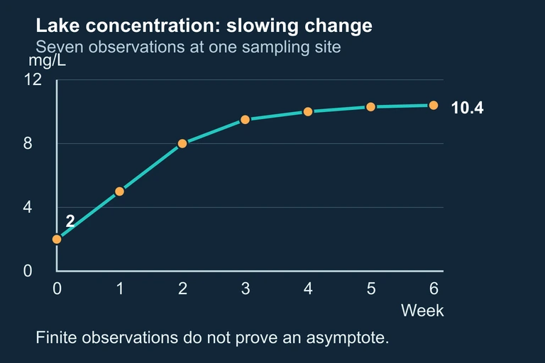Seven weekly observed nutrient concentrations: 2,5,8,9.5,10,10.3,10.4. Finite data show slowing but do not prove an asymptote. Seven observed lake concentrations suggest leveling within the observed window but cannot establish a unique horizontal asymptote.

SECTION 7

Strengths and Limitations of Each Model Family

No single function family is universally superior. Each model type has inherent strengths—contexts in which its assumptions align well with reality—and limitations—situations where its structural constraints cause it to misrepresent the data. The table below provides a side-by-side comparison that is especially useful when defending a model choice on free-response questions.

Model Family	Key Strengths	Key Limitations
Linear	Simplest model; fewest assumptions; excellent local approximation over short intervals; constant rate of change is easy to interpret.	Cannot model curvature, turning points, or bounded growth. Extrapolation often fails for large domains.
Quadratic	Models one turning point (max or min); constant second differences are easily verified; physically meaningful for projectile and area problems.	Symmetric parabolic shape may not match data; always unbounded for large \|x\|; cannot model asymptotic behavior.
Cubic / Higher Degree	Models multiple turning points and inflection; flexible shape; higher-degree polynomials can interpolate through any finite data set exactly.	Overfitting risk with higher degrees; wild oscillation between data points (Runge's phenomenon); strong assumptions needed for extrapolation.
Rational	Models asymptotic behavior (horizontal, vertical, slant); captures bounded growth and long-run limits; essential for rate and proportion problems.	Introduces discontinuities that may not exist in the physical context; more parameters to determine; domain restrictions must be contextually justified.

Comparison of polynomial and rational function families for model selection

✦

KEY TAKEAWAY

In engineering, every material specification sheet lists both the material's rated capacity and the conditions under which those ratings apply. Similarly, every function model comes with a "specification sheet" of assumptions. A linear model's spec sheet says "constant rate of change assumed"; a rational model's says "bounded output and excluded input values assumed." Your job on the AP exam is to read the data carefully, select the right "material," and then fill out the spec sheet by articulating those assumptions in your written response.

SECTION 8

Connections to Advanced Theory

The model selection skills you develop in AP Precalculus form the foundation for more sophisticated techniques encountered in calculus, statistics, and applied mathematics. The table below maps the precalculus concepts covered in this lesson to their more advanced counterparts, illustrating how assumption articulation becomes even more critical as models grow in complexity.

AP Precalculus Concept	Advanced Extension
Finite difference test for polynomial degree	Taylor polynomial approximation: nth-degree Taylor polynomials generalize finite differences to non-equally-spaced data via derivatives
Horizontal asymptote as long-run value	Formal limits at infinity in calculus; L'Hôpital's rule for indeterminate forms arising from rational expressions
Choosing between model families based on data	Statistical regression and model comparison using R², AIC, and BIC in AP Statistics and beyond
Articulating domain restrictions	Continuity and differentiability conditions in real analysis; piecewise function models in applied mathematics
Parsimony (prefer simpler model)	Occam's Razor formalized as the bias-variance tradeoff in machine learning; regularization techniques to prevent overfitting

Mapping precalculus model selection concepts to advanced mathematical frameworks

Looking forward, the habit of explicitly stating assumptions—"I chose a rational model because the data approach a limiting value, and I assume this limit exists because the physical context involves a saturation process"—transfers directly to writing scientific reports, engineering design documents, and statistical analyses. In each of these advanced contexts, the strength of a conclusion is only as strong as the clarity and validity of the assumptions that support it. Developing this disciplined approach now will serve you well in any quantitative field you pursue.

SECTION 9

Practice Problems

Question 1: CONCEPTUAL

A student claims that because a data set has five points, a degree-4 polynomial is the best model since it passes through all five points exactly. Which of the following best explains why this reasoning is flawed?

A. A degree-4 polynomial can only have four x-intercepts, so it cannot pass through five points.
B. Passing through all data points exactly does not mean the model captures the underlying relationship; the degree-4 polynomial may overfit the data by conforming to noise rather than the true trend, violating the principle of parsimony.
C. Degree-4 polynomials are undefined for certain values of x, making them unreliable models.
D. A degree-4 polynomial always has exactly four turning points, which is too many for most real-world data sets.
E. Polynomial models cannot be used unless the data have equally spaced inputs.

Show answer (B)

Correct: B. A polynomial of degree n − 1 can always be fit through n points exactly (the interpolation theorem), but exact fit does not imply an appropriate model. The principle of parsimony tells us to prefer the simplest model that captures the essential trend. A degree-4 polynomial forced through five points may oscillate wildly between data points (overfitting), producing poor predictions for inputs not in the data set. A is wrong because x-intercepts are not the same as data points—a polynomial can pass through points that are not on the x-axis. C is wrong because polynomials are defined for all real x. D is wrong because a degree-4 polynomial has at most 3 turning points, not exactly 4. E is wrong because polynomials can model data with unequal spacing; equally spaced inputs are required only for the finite difference test.

Question 2: BASIC CALCULATION

The following equally spaced data are given: | x | 0 | 2 | 4 | 6 | 8 | |---|---|---|---|---|---| | f(x) | 1 | 9 | 25 | 49 | 81 | Using the finite difference method, what is the degree of the polynomial that models this data?

A. 1 (linear)
B. 2 (quadratic)
C. 3 (cubic)
D. 4 (quartic)
E. The finite difference test cannot be applied because the step size is 2, not 1.

Show answer (B)

Correct: B. First differences (Δ¹): 9 − 1 = 8, 25 − 9 = 16, 49 − 25 = 24, 81 − 49 = 32. These are not constant, so the model is not linear. Second differences (Δ²): 16 − 8 = 8, 24 − 16 = 8, 32 − 24 = 8. The second differences are constant, indicating a quadratic (degree 2) polynomial. In fact, f(x) = (x + 1)² fits exactly: f(0) = 1, f(2) = 9, f(4) = 25, f(6) = 49, f(8) = 81. A is wrong because first differences are not constant. C and D overestimate the degree since constancy was achieved at the second level. E is wrong because the finite difference test works for any constant step size h; the inputs need only be equally spaced, and here h = 2.

Question 3: INTERMEDIATE

A rational function r(x) = (2x² + 3x − 5) / (x² − 4) has which of the following long-run behaviors and structural features?

A. Horizontal asymptote at y = 2, vertical asymptotes at x = 2 and x = −2, no holes.
B. Horizontal asymptote at y = 0, vertical asymptotes at x = 2 and x = −2, no holes.
C. Slant asymptote y = 2x + 3, vertical asymptotes at x = 2 and x = −2.
D. Horizontal asymptote at y = 2, vertical asymptote at x = −2 only, with a hole at x = 2.
E. Horizontal asymptote at y = 2, vertical asymptote at x = 2 only, with a hole at x = −2.

Show answer (A)

Correct: A. Since the numerator and denominator have equal degree (both degree 2), the horizontal asymptote is y = (leading coefficient of numerator)/(leading coefficient of denominator) = 2/1 = 2. The denominator factors as (x − 2)(x + 2), giving potential vertical asymptotes or holes at x = 2 and x = −2. Checking the numerator: 2x² + 3x − 5 = (2x + 5)(x − 1). Since neither (x − 2) nor (x + 2) is a factor of the numerator, no cancellation occurs, so both are vertical asymptotes with no holes. B is wrong because y = 0 is the HA only when deg(numerator) < deg(denominator). C is wrong because slant asymptotes occur only when deg(numerator) = deg(denominator) + 1. D and E are wrong because neither (x − 2) nor (x + 2) cancels with a factor of the numerator, so no hole exists.

Question 4: APPLIED

7 pts

A pharmaceutical company measures the concentration C(t) of a drug in a patient's bloodstream (in mg/L) at times t = 0, 1, 2, 3, 4, 5 hours after administration. The recorded values are: t: 0, 1, 2, 3, 4, 5 C(t): 0, 4.8, 5.0, 4.0, 3.0, 2.2 (a) Explain why a polynomial model of degree 3 or higher might be appropriate for this data. Identify the specific features of the data that support this claim. (b) A researcher proposes the rational model C(t) = at/(t² + b) instead. Explain the pharmacological assumption embedded in this model, and describe one advantage this model has over a cubic polynomial for predicting drug concentration at t = 10 hours. (c) Using the rational model C(t) = at/(t² + b), find the values of a and b given that C(1) = 4.8 and C(2) = 5.0. (d) State the horizontal asymptote of your model from part (c) and explain its real-world meaning.

Show answer

Rubric (7 points): Part (a) — 2 points: (1 pt) The data rise from 0 to a maximum near t = 2, then decrease, indicating at least one local maximum—a feature requiring degree ≥ 2. (1 pt) Because the data also appear to have an inflection (concave up then concave down, or vice versa) and the function starts at 0, rises, peaks, and falls, a cubic polynomial can model the rise-peak-fall shape with the necessary inflection point. Part (b) — 2 points: (1 pt) The rational model C(t) = at/(t² + b) embeds the pharmacological assumption that the drug concentration rises quickly after administration and then decays toward zero as the body metabolizes and eliminates the drug. The horizontal asymptote at y = 0 captures the idea that over a long time, the drug is fully cleared. (1 pt) At t = 10, a cubic polynomial would likely produce a large negative value (since cubics tend toward −∞ or +∞), which is physically impossible for concentration. The rational model, by contrast, yields a small positive value approaching 0, which is biologically realistic. Part (c) — 2 points: (1 pt) From C(1) = 4.8: a(1)/(1 + b) = 4.8, so a = 4.8(1 + b). From C(2) = 5.0: 2a/(4 + b) = 5.0, so 2a = 5(4 + b), giving a = (20 + 5b)/2. (1 pt) Setting equal: 4.8(1 + b) = (20 + 5b)/2 → 9.6 + 9.6b = 20 + 5b → 4.6b = 10.4 → b ≈ 2.26. Then a = 4.8(1 + 2.26) = 4.8 × 3.26 ≈ 15.65. So C(t) ≈ 15.65t/(t² + 2.26). Part (d) — 1 point: (1 pt) The horizontal asymptote is y = 0, because the degree of the numerator (1) is less than the degree of the denominator (2). In real-world terms, this means that as time passes, the drug concentration in the bloodstream approaches zero—the drug is fully metabolized and eliminated from the body.

Question 5: CRITICAL THINKING

4 pts

A classmate presents the following argument: "Since any continuous function on a closed interval can be uniformly approximated by a polynomial (the Weierstrass Approximation Theorem), polynomial models are always sufficient, and we never need rational function models." (a) Identify the logical flaw in this argument as it relates to model selection in precalculus. (b) Provide a specific real-world scenario where a rational model is structurally necessary and explain which assumption of the polynomial model is violated. (c) Explain how the principle of parsimony applies to this debate.

Show answer

Rubric (4 points): Part (a) — 1 point: (1 pt) The Weierstrass theorem guarantees approximation on a closed, bounded interval [a, b], but modeling often requires extrapolation beyond observed data and behavior on unbounded domains. Polynomials grow without bound as x → ±∞, so they cannot capture the asymptotic leveling-off or bounded behavior that many real-world phenomena exhibit. A good model must not only approximate known data but also encode structural features (like asymptotes) that govern behavior outside the observed range. Part (b) — 2 points: (1 pt) Example: the concentration of a chemical reaction approaching equilibrium. As time increases, the concentration approaches a fixed saturation level (horizontal asymptote), and the reaction rate depends on a ratio of quantities—both features that demand a rational model. (1 pt) The polynomial assumption that is violated is continuity of growth: polynomials of odd degree grow without bound, and polynomials of even degree grow to +∞ on both ends (or −∞ on both ends). Neither behavior matches a bounded concentration approaching a finite limit. Part (c) — 1 point: (1 pt) Parsimony favors the model that captures the essential behavior with the fewest parameters and weakest assumptions. While a high-degree polynomial could approximate bounded data on a given interval, it would require many parameters and impose the strong (and violated) assumption of unbounded end behavior. A rational function with 3–4 parameters naturally encodes the asymptotic structure, making it both simpler in assumption and more appropriate structurally. The parsimonious choice is the rational model because its built-in assumptions match the physics of the situation.

SUMMARY

Lesson Summary

Summary

Function model selection requires you to match data behavior to the structural properties of a function family. Begin by examining end behavior: does the output grow without bound (polynomial) or approach a horizontal asymptote (rational)? Next, apply the finite difference test to equally spaced data to identify the polynomial degree: constant first differences signal linear, constant second differences signal quadratic, and so on. For rational models, compare the degrees of the numerator and denominator to determine the asymptotic structure, and verify that the data support the existence of excluded input values.

Equally important is assumption articulation: every model carries embedded assumptions about continuity, rate of change patterns, domain restrictions, and end behavior that must be explicitly stated and defended with evidence from the data or the problem's real-world context. Adhere to the principle of parsimony—choose the simplest model whose assumptions are satisfied—and always check that your model's behavior is physically or contextually reasonable, especially for extrapolation beyond the observed data range. Mastering this synthesis of quantitative analysis and verbal justification is a cornerstone of success on the AP Precalculus exam.