

SECTION 1
Historical Context & Motivation
The study of conic sections ranks among the oldest investigations in mathematics, originating in ancient Greece and persisting as one of the most consequential topics in analytic geometry. These curves—circles, ellipses, parabolas, and hyperbolas—arise naturally when a plane intersects a double-napped cone at various angles. Greek geometers initially studied conics for their intrinsic beauty, but the curves later proved indispensable for describing planetary orbits, projectile trajectories, and the behavior of light and sound. In the modern AP Precalculus curriculum, conic sections serve as a bridge between algebraic equations, parametric representations, and matrix transformations, making them a natural testing ground for the unit on parameters, vectors, and matrices.
~350 BCE • Menaechmus & the Double Cone
~200 BCE • Apollonius of Perga
1609 • Kepler's Elliptical Orbits
1637 • Descartes & Analytic Geometry
The central question that conic sections answer is deceptively simple: how can a single family of second-degree equations describe such diverse shapes, and how do parametric equations and matrix operations let us manipulate, rotate, and translate these curves with precision? Mastering conics equips you with the algebraic and geometric fluency needed for calculus, physics, and engineering.
SECTION 2
Core Principles & Definitions
Every conic section can be understood as the set of points satisfying a specific geometric relationship involving distances to fixed elements—a focus (a fixed point) and a directrix (a fixed line). The ratio of the distance from any point on the curve to the focus versus its distance to the directrix is the eccentricity (e), and this single parameter determines the conic's type. Equivalently, conics are defined as the intersection of a plane with a right circular double cone—the angle of the cutting plane relative to the cone's axis determines which curve results.
Circle (e = 0)
Ellipse (0 < e < 1)
Parabola (e = 1)
Hyperbola (e > 1)
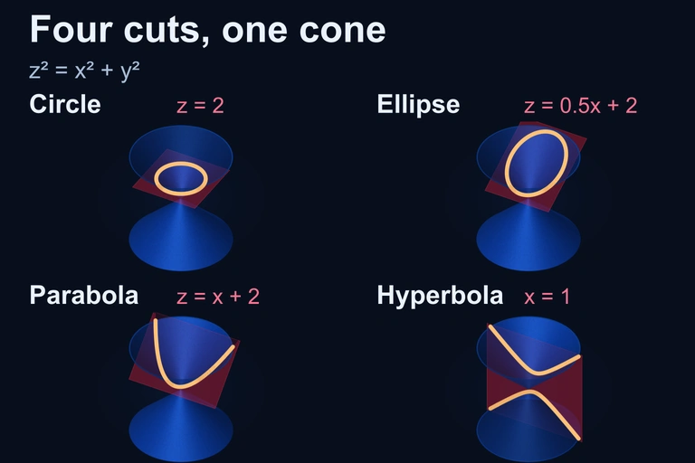 Four cone-plane intersections: circle for z=2, ellipse for z=0.5x+2, parabola for z=x+2 and hyperbola for x=1.
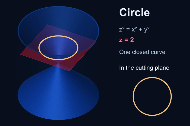 Horizontal plane z=2 cuts one cone nappe in a circle, with a plane-normal circular view.
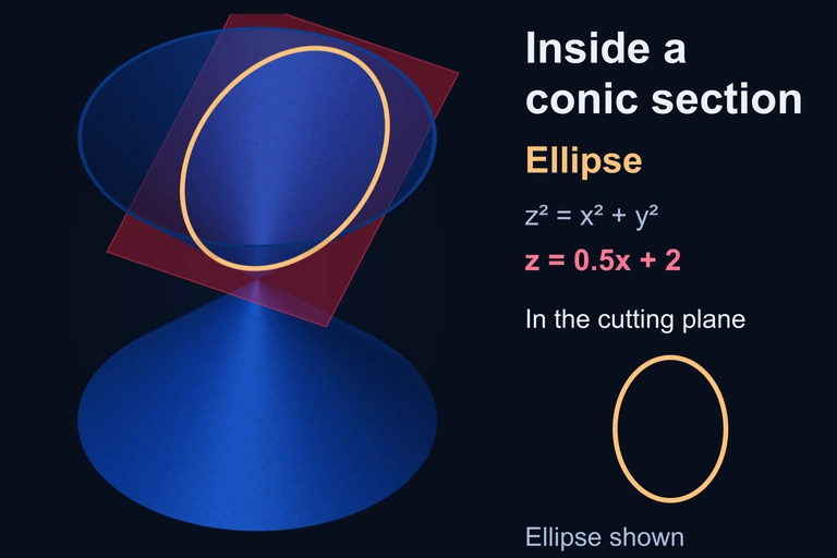
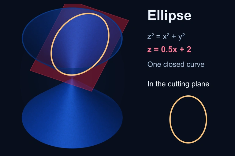 Oblique plane z=0.5x+2 cuts one cone nappe in a closed ellipse, with a plane-normal view.
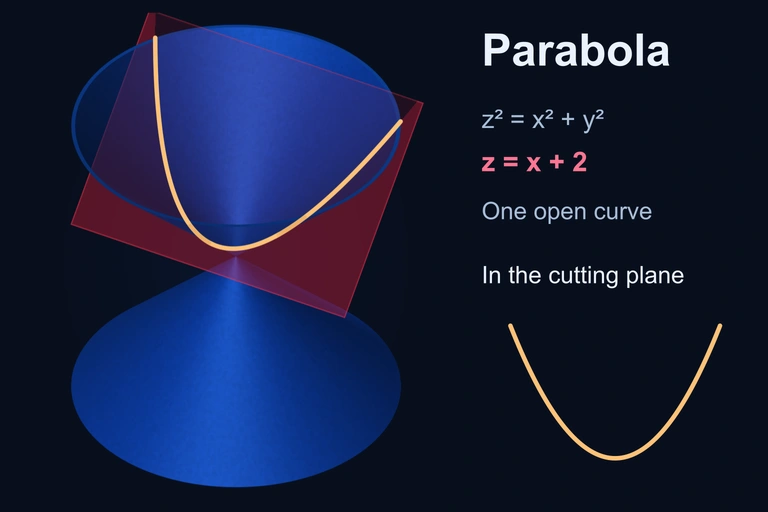 Plane z=x+2, parallel to a cone generator, gives an open parabola. The finite render boundary does not close the curve.
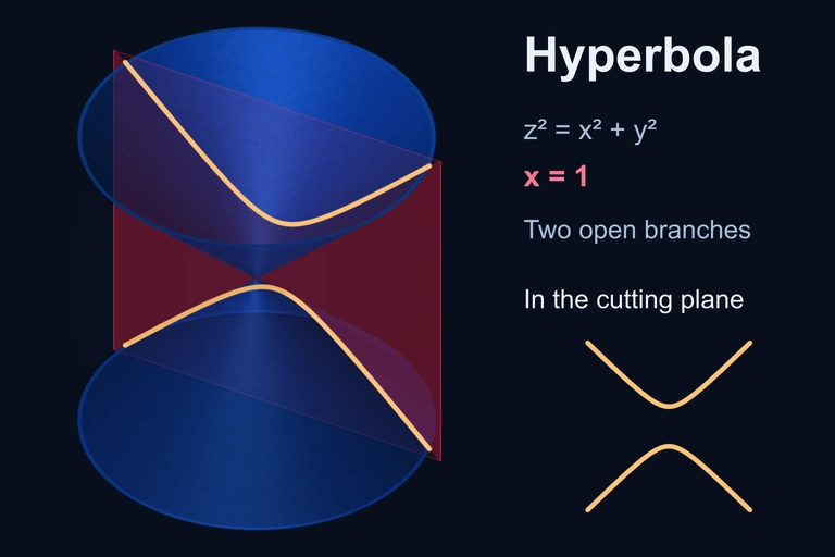 Vertical plane x=1 cuts both cone nappes in two hyperbola branches, with a plane-normal view.
SECTION 3
Visualizing the Conic Family
Notice how the geometric elements—center, foci, directrix, and axes of symmetry—shift as eccentricity changes. In the circle, the single center is the lone defining point. The ellipse introduces two foci that sit along the major axis; the closer they are together, the more circular the ellipse appears. The parabola's single focus and directrix work in tandem: every point on the curve is equidistant from both. Finally, the hyperbola's two branches curve away from each other, each approaching but never touching a pair of asymptotes. Being comfortable reading these visual features is essential before translating them into algebraic and parametric forms.
SECTION 4
Mathematical Framework
Standard Forms of Conics (Center at Origin)
GENERAL SECOND-DEGREE EQUATION
Every conic can be expressed in this form. The discriminant B² − 4AC classifies the conic: < 0 → ellipse/circle, = 0 → parabola, > 0 → hyperbola.
ELLIPSE (a > b)
Semi-major axis a along the x-axis, semi-minor axis b along the y-axis. Foci at (±c, 0) where c² = a² − b². When a = b, this becomes a circle of radius a.
HYPERBOLA (HORIZONTAL TRANSVERSE AXIS)
Opens left-right. Vertices at (±a, 0), foci at (±c, 0) where c² = a² + b². Asymptotes: y = ±(b/a)x.
PARABOLA (VERTICAL AXIS)
Focus at (0, p), directrix at y = −p. If p > 0 the parabola opens upward; if p < 0 it opens downward. The analogous horizontal form is y² = 4px.
Parametric Representations
In the AP Precalculus context of parametric functions, conics can be traced by expressing x and y each as functions of a parameter t. For an ellipse with semi-axes a and b, the standard parametric form is x(t) = a cos t, y(t) = b sin t for t ∈ [0, 2π). For a hyperbola, we use x(t) = a sec t, y(t) = b tan t. These parametric forms are essential for eliminating the parameter to recover the rectangular equation, a core AP Precalculus skill. Rotation of conics by an angle θ can be handled by applying a rotation matrix to the parametric vector ⟨x(t), y(t)⟩, connecting this topic directly to the matrices strand of the course.
SECTION 5
Detailed Classification & the Discriminant
Given the general second-degree equation Ax² + Bxy + Cy² + Dx + Ey + F = 0, the value of the conic discriminant Δ = B² − 4AC provides a quick classification without completing the square or graphing. This quantity is invariant under rotation of axes, meaning it yields the same conic type regardless of orientation. The table below summarizes the classification alongside key geometric elements for each type.
| Conic | Discriminant Δ | Eccentricity | Key Relationship |
|---|---|---|---|
| Circle | < 0 (and A = C, B = 0) | e = 0 | All points equidistant from center |
| Ellipse | < 0 (A ≠ C or B ≠ 0) | 0 < e < 1 | Sum of distances to foci = 2a |
| Parabola | = 0 | e = 1 | Distance to focus = distance to directrix |
| Hyperbola | > 0 | e > 1 | |Difference of distances to foci| = 2a |
Classification of conics by discriminant and eccentricity
SECTION 6
Worked Example: Identifying & Parametrizing an Ellipse
Consider the equation 9x² + 25y² − 54x + 100y − 44 = 0. We will classify this conic, rewrite it in standard form, identify its key features, and express it parametrically.
Worked example
- 1
Step 1 — Apply the Discriminant Test
Here A = 9, B = 0, C = 25. Compute Δ = B² − 4AC = 0 − 4(9)(25) = −900. Since Δ < 0 and A ≠ C, the conic is an ellipse.Δ = −900 → Ellipse - 2
Step 2 — Group and Complete the Square
Group x-terms and y-terms: 9(x² − 6x) + 25(y² + 4y) = 44. Complete each square: 9(x² − 6x + 9) + 25(y² + 4y + 4) = 44 + 81 + 100 = 225. This yields 9(x − 3)² + 25(y + 2)² = 225.9(x − 3)² + 25(y + 2)² = 225 - 3
Step 3 — Write in Standard Form
Divide both sides by 225: (x − 3)²/25 + (y + 2)²/9 = 1. We read off a² = 25 so a = 5, b² = 9 so b = 3. The center is (h, k) = (3, −2). Since a > b and a is under the x-term, the major axis is horizontal.(x − 3)²/25 + (y + 2)²/9 = 1, center (3, −2) - 4
Step 4 — Find Foci and Eccentricity
Compute c² = a² − b² = 25 − 9 = 16, so c = 4. Foci lie along the major axis at (3 ± 4, −2), giving (7, −2) and (−1, −2). Eccentricity e = c/a = 4/5 = 0.8.Foci: (7, −2) and (−1, −2); e = 0.8 - 5
Step 5 — Write Parametric Equations
Using x = h + a cos t and y = k + b sin t, we obtain x(t) = 3 + 5 cos t and y(t) = −2 + 3 sin t for t ∈ [0, 2π). We can verify by eliminating the parameter: cos t = (x − 3)/5 and sin t = (y + 2)/3, and since cos²t + sin²t = 1, we recover the standard form.x(t) = 3 + 5 cos t, y(t) = −2 + 3 sin t, t ∈ [0, 2π)
SECTION 7
Comparing Representations: Rectangular, Parametric, and Polar
Conics can be represented in rectangular (Cartesian) form, parametric form, and polar form. Each representation has strengths depending on the task—whether you need to graph, compute arc length, rotate the curve, or analyze orbital mechanics. Understanding when to convert between forms is a central AP Precalculus skill.
| Representation | Strengths | Limitations |
|---|---|---|
| Rectangular | Direct algebraic manipulation; discriminant classification; completing the square identifies center and axes immediately. | Cannot represent direction of traversal; rotated conics produce messy Bxy cross-terms; not easily parameterized for calculus. |
| Parametric | Shows direction and speed of traversal; easy to apply rotation matrices; eliminates multi-valued y issues for vertical lines. | Requires eliminating the parameter to recover the Cartesian equation; choice of parameter is not unique. |
| Polar | Elegantly unifies all conics via r = ed/(1 ± e cos θ); natural for orbital mechanics; eccentricity appears explicitly. | Requires focus at the origin; not convenient for conics centered elsewhere without translation. |
Comparison of conic representations
SECTION 8
Connection to Calculus, Matrices, and Beyond
Conic sections serve as a gateway to several advanced topics. In AP Calculus BC, parametric derivatives dy/dx = (dy/dt)/(dx/dt) allow you to find tangent lines and arc lengths of conics without ever solving for y explicitly. In linear algebra, the general second-degree equation corresponds to a quadratic form vTMv = 0, where M is a symmetric 2 × 2 matrix whose eigenvalues determine the conic type. Diagonalizing M is equivalent to rotating axes to eliminate the Bxy cross-term—an elegant connection to the matrices strand of this AP unit.
| AP Precalculus Topic | Advanced Extension |
|---|---|
| Parametric equations of conics | Parametric derivatives, arc length, and surface area of revolution in Calculus BC |
| Discriminant B² − 4AC | Eigenvalues of the associated matrix; quadratic form classification in linear algebra |
| Rotation of conic axes | Orthogonal diagonalization; principal axis theorem |
| Polar form r = ed/(1 ± e cos θ) | Kepler's laws; gravitational orbits; astrophysics trajectory calculations |
From AP Precalculus to advanced topics
For now, focus on building fluency with the standard forms, parametric representations, and the discriminant test. These skills form the foundation upon which all advanced treatments—whether in multivariable calculus, differential equations, or physics—are built.
SECTION 9
Practice Problems
Question 1: CONCEPTUAL
- A. Parabola
- B. Ellipse (not a circle)
- C. Circle
- D. Hyperbola
- E. Degenerate conic (a single point)
Show answer (C)
Question 2: BASIC CALCULATION
- A. √7
- B. 2√7
- C. 5
- D. 7
- E. 10
Show answer (B)
Question 3: INTERMEDIATE
- A. Ellipse with e < 1
- B. Parabola with e = 1
- C. Hyperbola with e > 1
- D. Circle with e = 0
- E. Cannot be determined without eliminating the cross-term
Show answer (C)
Question 4: APPLIED
Show answer
Question 5: CRITICAL THINKING