Competing Function Model Validation - AP Precalculus

SECTION 1

Historical Context & Motivation

The question of how to choose the right mathematical model for a data set is as old as the scientific method itself. When scientists first began collecting systematic measurements—population counts, radioactive decay readings, financial records—they faced a fundamental challenge: multiple function families can appear to fit the same data over a limited domain. A linear model, a quadratic model, and an exponential model might all seem reasonable when you only have five or six data points clustered in a narrow interval. Competing function model validation is the systematic process of testing rival function types against data to determine which one captures the underlying relationship most faithfully.

1805 • Least Squares Method

Adrien-Marie Legendre published the method of least squares, giving mathematicians a formal criterion for measuring how well a model fits observed data.

1838 • Verhulst's Logistic Model

Pierre-François Verhulst proposed the logistic growth model as a competitor to Malthus's purely exponential population model, illustrating the need to compare rival function families.

1900s • Residual Analysis Emerges

Statisticians formalized residual plots as diagnostic tools, enabling analysts to visually detect systematic misfit and choose between competing models.

2000s • AP Curriculum Integration

The College Board embedded model selection and validation into AP Precalculus and AP Statistics, requiring students to justify why one function type is more appropriate than another.

The central question this lesson addresses is deceptively simple: given a data set, how do you decide whether a linear, quadratic, exponential, or logarithmic model is most appropriate? The answer requires you to move beyond curve-fitting intuition and employ structural tests—analyzing rates of change, residual patterns, and end behavior to discriminate among competing models.

SECTION 2

Core Principles of Model Validation

Model validation rests on a few foundational ideas that connect algebraic structure to data behavior. Each function family—linear, quadratic, exponential, logarithmic—has a unique algebraic signature that manifests in the data's first and second differences, ratios, and long-run trends. Understanding these signatures allows you to match the right model to the data without relying on graphing calculator regression alone.

Constant Rate of Change → Linear

If consecutive outputs change by roughly the same amount for equal input increments, the data is linear: f(x) = mx + b. Check that first differences Δy are approximately constant.

Constant Second Differences → Quadratic

If first differences themselves change at a constant rate, the data is quadratic: f(x) = ax² + bx + c. The second differences Δ²y should be approximately constant.

Constant Ratio → Exponential

If consecutive outputs are related by a nearly constant multiplicative factor for equal input steps, the data is exponential: f(x) = a · bˣ. Check that ratios y₍ₙ₊₁₎ / yₙ are approximately constant.

Residual Analysis

After fitting a candidate model, compute residuals (observed − predicted). If residuals show a random scatter, the model is appropriate. A curved pattern in residuals signals systematic misfit.

End Behavior & Domain Constraints

Evaluate whether the model's long-run behavior matches the context. Exponential models grow without bound; logarithmic models increase slowly; linear models lack curvature. Physical context may rule out certain families.

SECTION 3

Visual Explanation: Comparing Models on One Data Set

Three candidate models—linear (blue dashed), exponential (violet solid), and quadratic (green dotted)—are overlaid on the same data points. Notice how the linear model diverges substantially from the data at the extremes, while the exponential and quadratic models track more closely. The next step is to examine residuals to distinguish between the two curved models.

The diagram above illustrates a core challenge in model validation: over a restricted domain, multiple function families can approximate the data reasonably well. The linear model (blue dashed line) captures the general upward trend but systematically undershoots on the right side, where the data curves upward more steeply. Both the exponential and quadratic curves hug the data points more tightly, but they diverge from each other outside the observed range. To distinguish between these two, you need to apply the algebraic signature tests—checking whether successive output ratios or successive second differences are approximately constant—and then examine the residuals for systematic patterns.

SECTION 4

Mathematical Framework for Model Selection

The mathematical backbone of model validation consists of difference and ratio tests applied to equally spaced input values. Suppose you have data points (x₁, y₁), (x₂, y₂), …, (xₙ, yₙ) where the x-values are equally spaced with common increment Δx. The following tests let you classify the underlying function.

FIRST DIFFERENCES (LINEAR TEST)

Δyₖ = yₖ₊₁ − yₖ

If all Δyₖ are approximately equal, the data is linear. The common difference equals m · Δx, where m is the slope.

SECOND DIFFERENCES (QUADRATIC TEST)

Δ²yₖ = Δyₖ₊₁ − Δyₖ

If first differences are not constant but second differences Δ²yₖ are approximately constant, the data is quadratic. The constant second difference equals 2a · (Δx)², where a is the leading coefficient.

CONSECUTIVE RATIOS (EXPONENTIAL TEST)

rₖ = yₖ₊₁ / yₖ

If all rₖ are approximately equal and positive, the data is exponential. The common ratio equals $b^{Δx}$ , where b is the base of f(x) = a · bˣ.

RESIDUAL

eₖ = yₖ(observed) − yₖ(predicted)

After fitting a candidate model, compute residuals for each data point. A good fit produces residuals that are small in magnitude, randomly scattered, and show no systematic pattern when plotted against x.

ℹ

AP Exam Tip

SECTION 5

Algebraic Signatures of Each Function Family

Each function family leaves a distinctive algebraic fingerprint in equally spaced data. The table below summarizes these signatures alongside the corresponding end behavior and contextual clues that help you narrow down the correct model on the AP exam.

Model	Form	Data Signature	End Behavior
Linear	f(x) = mx + b	Constant first differences	→ ±∞ as x → ±∞
Quadratic	f(x) = ax² + bx + c	Constant second differences	Both ends → +∞ or both → −∞
Exponential	f(x) = a · bˣ (b > 0, b ≠ 1)	Constant consecutive ratios	One end → 0, other → ∞
Logarithmic	f(x) = a + b · ln(x)	Decreasing differences; inputs with constant ratios yield constant output differences	→ ∞ slowly as x → ∞; undefined for x ≤ 0

Summary of algebraic signatures for the four major AP Precalculus function families

This decision flowchart guides you through the sequence of tests to apply when given equally spaced data. Start by checking first differences; if they fail, test ratios for exponential behavior; if those also fail, check second differences for a quadratic pattern. If none of these tests yields approximately constant values, consider a logarithmic or other specialized model.

A special note on logarithmic models: because logarithmic and exponential functions are inverses, the logarithmic signature is essentially the exponential test applied to the roles of x and y reversed. If your input values have a constant ratio and the output differences are approximately constant, the data follows a logarithmic pattern. This situation arises naturally in contexts like the Richter scale, decibel measurements, and pH.

SECTION 6

Worked Example: Choosing Between Exponential and Quadratic

Consider the following data set collected from a biological experiment measuring the number of bacteria (in thousands) in a culture over equally spaced time intervals.

t (hours)	0	1	2	3	4	5
N(t)	5	10	20	39	80	158

Bacteria population data (thousands)

Worked example

1
Step 1 — Compute First Differences

Δy: 10 − 5 = 5, 20 − 10 = 10, 39 − 20 = 19, 80 − 39 = 41, 158 − 80 = 78. The first differences are 5, 10, 19, 41, 78—clearly not constant, so no linear function passes exactly through all six observations.

No exact linear fit — first differences vary.
2
Step 2 — Compute Consecutive Ratios

r: 10/5 = 2.00, 20/10 = 2.00, 39/20 = 1.95, 80/39 ≈ 2.05, 158/80 ≈ 1.975. All ratios are approximately 2.0, suggesting an exponential model with base b ≈ 2.

Ratios ≈ 2.0 — strong exponential signal.
3
Step 3 — Check Second Differences (Competing Test)

Δ²y: 10 − 5 = 5, 19 − 10 = 9, 41 − 19 = 22, 78 − 41 = 37. The second differences are 5, 9, 22, 37—these are not constant, so no quadratic function passes exactly through all six observations.

No exact quadratic fit — second differences vary.
4
Step 4 — Propose an Exponential Model and Examine Residuals

Using N(0) = 5 and the near-constant ratio 2, propose N(t) = 5·2ᵗ. Predictions are 5, 10, 20, 40, 80, 160, with residuals 0, 0, 0, −1, 0, −2. This candidate fits closely over the observed interval, but six small residuals do not establish uniqueness, a patternless error process, or future accuracy. The supplemental curves 5 + 31t and 5 + 6t² are illustrative comparators, not least-squares fits.

N(t) = 5·2ᵗ fits closely here; further validation is needed.

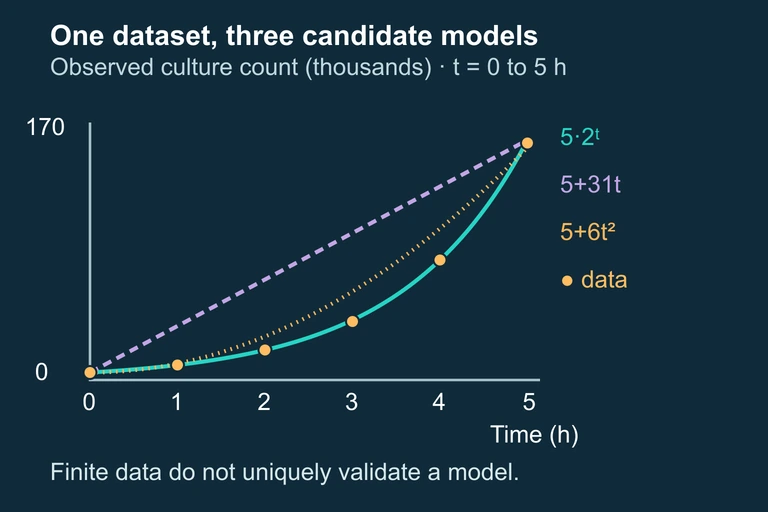Six observed values plotted with three named model candidates. The exponential candidate follows the observations closely over the displayed interval. The selected exponential model leaves residuals 0,0,0,−1,0,−2; a few small residuals support comparison but do not prove a model.

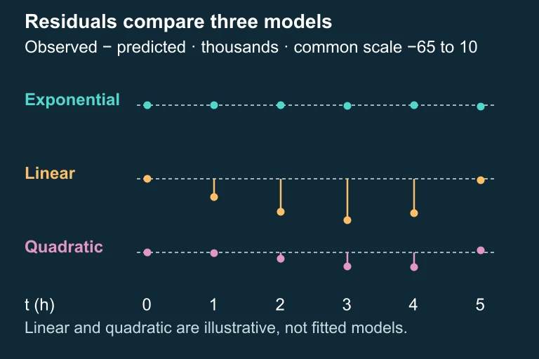Three residual plots on a common vertical scale. The linear and quadratic curves are illustrative comparisons rather than fitted models.

★

Key takeaway

VALIDATION STRATEGY

A researcher looks through a microscope beside a closed culture vessel,sample containers and an illustrative cell inset. For the six observations 5, 10, 20, 39, 80, and 158 thousand, the model N = 5×2^t gives residuals 0, 0, 0, −1, 0, and −2 thousand.

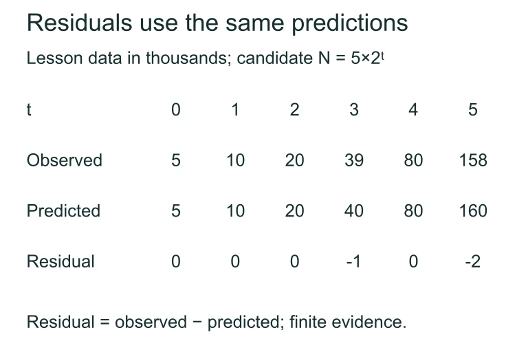For the six observations 5, 10, 20, 39, 80, and 158 thousand, the model N = 5×2^t gives residuals 0, 0, 0, −1, 0, and −2 thousand.

SECTION 7

Strengths & Limitations of Each Model Type

No single function family is universally superior; each has contexts where it excels and contexts where it fails. The table below compares the four primary AP Precalculus models across several practical dimensions that the exam frequently tests.

Criterion	Linear	Quadratic	Exponential	Logarithmic
Short-term fit	Good over narrow intervals	Good with curvature	Good for growth/decay	Good for rapid-then-slow
Extrapolation risk	Moderate (no curvature)	High (unbounded both ends)	Very high (grows to ∞)	Low (slow growth)
Domain restrictions	All real numbers	All real numbers	All reals (output > 0 if a > 0)	x > 0 only
Common misfit signal	Curved residual plot	Residuals grow at extremes	Overpredicts when growth slows	Underpredicts for large x if growth continues

Comparison of model types across common validation criteria

★

Key takeaway

CONTEXT MATTERS

SECTION 8

Connection to Advanced Regression & AP Statistics

The model validation techniques you learn in AP Precalculus form the conceptual bridge to more advanced topics in AP Statistics and college-level data analysis. While Precalculus focuses on algebraic signatures (differences, ratios) and qualitative residual analysis, statistics courses formalize these ideas with numerical diagnostics like the coefficient of determination (R²), information criteria, and hypothesis tests on residuals.

AP Precalculus Approach	Advanced / AP Statistics Extension
Check first differences, second differences, and ratios	Linearize the model (e.g., log-transform) and compute R² for each candidate
Visually inspect residual plots for patterns	Run formal residual diagnostics: Durbin-Watson test, runs test for randomness
Use context and end behavior to eliminate candidates	Apply Akaike Information Criterion (AIC) to penalize model complexity
Fit model by matching initial value and common ratio or slope	Least-squares regression with transformed variables (e.g., ln y vs. x for exponential)

How Precalculus model validation connects to advanced regression

One powerful technique that bridges both courses is linearization. If you suspect an exponential model y = a · bˣ, taking the natural logarithm of both sides yields ln y = ln a + x · ln b, which is linear in x. If a scatter plot of (x, ln y) is approximately linear, the original data is exponential. This same strategy validates power models (use ln y vs. ln x) and is a cornerstone of AP Statistics regression analysis.

ℹ

Looking Ahead

SECTION 9

Practice Problems

Question 1: CONCEPTUAL

A data set of equally spaced x-values produces the following first differences: 12, 12.1, 11.9, 12, 12.1. Which of the following function types best models this data? (A) Quadratic (B) Exponential growth (C) Linear (D) Logarithmic (E) Exponential decay

A. Quadratic
B. Exponential growth
C. Linear
D. Logarithmic
E. Exponential decay

Show answer (C)

The correct answer is (C) Linear. The first differences are approximately constant (all near 12), which is the defining algebraic signature of a linear function. (A) is incorrect because a quadratic model requires constant second differences, not constant first differences. (B) and (E) are incorrect because exponential models are identified by constant consecutive ratios, not constant differences. (D) is incorrect because logarithmic data would show decreasing first differences as x increases.

Question 2: BASIC CALCULATION

Given the data: x = 0, 1, 2, 3, 4 and y = 3, 9, 27, 81, 243, which of the following is the best model for this data? (A) y = 3x + 3 (B) y = 2 · 3ˣ (C) y = 3 · 3ˣ (D) y = 3x² (E) y = 3 · ln(x + 1)

A. y = 3x + 3
B. y = 2 · 3ˣ
C. y = 3 · 3ˣ
D. y = 3x²
E. y = 3 · ln(x + 1)

Show answer (C)

The correct answer is (C) y = 3 · 3ˣ. Computing consecutive ratios: 9/3 = 3, 27/9 = 3, 81/27 = 3, 243/81 = 3. The constant ratio of 3 identifies this as exponential with base b = 3. At x = 0, y = 3, so a = 3, giving y = 3 · 3ˣ. (A) is incorrect because a linear model would require constant differences, but differences here are 6, 18, 54, 162—not constant. (B) is incorrect: 2 · 3ˣ at x = 0 gives 2 ≠ 3, so it fails the first data point. (D) is incorrect: 3(1)² = 3, but 3(2)² = 12 ≠ 27. (E) is incorrect: logarithmic functions increase slowly and cannot produce the rapid growth seen here.

Question 3: INTERMEDIATE

The table below shows data collected from an experiment. x: 1 2 3 4 5 6 y: 2 8 18 32 50 72 A student claims the data is exponential because the y-values are increasing rapidly. Which of the following best explains why the student is incorrect? (A) The first differences are constant, indicating a linear model. (B) The consecutive ratios are not approximately constant; the second differences are constant at 4, indicating a quadratic model. (C) The data has a vertical asymptote, indicating a logarithmic model. (D) The consecutive ratios equal 2, confirming an exponential model. (E) The second differences are increasing, so a cubic model is needed.

A. The first differences are constant, indicating a linear model.
B. The consecutive ratios are not approximately constant; the second differences are constant at 4, indicating a quadratic model.
C. The data has a vertical asymptote, indicating a logarithmic model.
D. The consecutive ratios equal 2, confirming an exponential model.
E. The second differences are increasing, so a cubic model is needed.

Show answer (B)

The correct answer is (B). First differences: 6, 10, 14, 18, 22—not constant, so not linear (eliminating A). Second differences: 4, 4, 4, 4—constant, which is the signature of a quadratic model. Consecutive ratios: 8/2 = 4, 18/8 = 2.25, 32/18 ≈ 1.78, 50/32 ≈ 1.56—these are not constant, disproving the exponential claim and eliminating (D). The data is y = 2x², which is quadratic. (C) is wrong because logarithmic models are not suggested by this data's behavior. (E) is wrong because the second differences are constant, not increasing.

Question 4: APPLIED

A pharmaceutical researcher measures the concentration C (mg/L) of a drug in a patient's bloodstream at one-hour intervals after administration: t (hours): 0, 1, 2, 3, 4, 5 C(t): 200, 140, 98, 68.6, 48, 33.7 (a) Compute the consecutive ratios and determine whether a linear or exponential model is more appropriate. Justify your answer. (b) Write an exponential model of the form C(t) = a · bᵗ using the initial concentration and the average ratio. (c) Use your model to predict the concentration at t = 8 hours. (d) The drug is considered ineffective below 10 mg/L. Using your model, estimate when the concentration drops below this threshold.

Show answer

(a) [2 points] Consecutive ratios: 140/200 = 0.70, 98/140 = 0.70, 68.6/98 = 0.70, 48/68.6 ≈ 0.70, 33.7/48 ≈ 0.70. All ratios are approximately 0.70. Since the ratios are constant, the data is exponential rather than linear. First differences would be −60, −42, −29.4, −20.6, −14.3—these are not constant, further confirming that linear is inappropriate. (b) [1 point] Using a = C(0) = 200 and b ≈ 0.70: C(t) = 200 · (0.70)ᵗ. (c) [1 point] C(8) = 200 · (0.70)⁸ = 200 · 0.0576 ≈ 11.5 mg/L. (d) [2 points] Solve 200 · (0.70)ᵗ = 10. Dividing: (0.70)ᵗ = 0.05. Taking ln of both sides: t · ln(0.70) = ln(0.05), so t = ln(0.05)/ln(0.70) = (−2.996)/(−0.357) ≈ 8.4 hours. The concentration drops below 10 mg/L at approximately t ≈ 8.4 hours.

Question 5: CRITICAL THINKING

A student fits both an exponential model f(x) = 2 · (1.5)ˣ and a quadratic model g(x) = 0.8x² + 1.2 to a data set. The residuals for each model are given below: Exponential residuals: −0.1, 0.3, −0.2, 0.1, 0.0, −0.2 Quadratic residuals: −0.5, 0.8, −0.9, 1.1, −1.3, 1.5 (a) For each model, describe the pattern (or lack thereof) in the residuals. (b) Based on the residuals, determine which model is more appropriate and justify your reasoning. (c) Explain why a model can have a smaller sum of residuals yet still be the worse choice.

Show answer

(a) [1 point] The exponential residuals (−0.1, 0.3, −0.2, 0.1, 0.0, −0.2) are small in magnitude and show no systematic pattern—they alternate signs randomly and stay close to zero. The quadratic residuals (−0.5, 0.8, −0.9, 1.1, −1.3, 1.5) alternate in sign but their magnitudes are increasing, suggesting a systematic pattern where the model's error grows with x. (b) [1 point] The exponential model is more appropriate. Its residuals are both smaller in magnitude and randomly scattered, indicating that f(x) = 2 · (1.5)ˣ captures the data's structure without systematic misfit. The quadratic residuals show a growing oscillation that signals the model is not capturing the underlying trend. (c) [1 point] The sum of residuals can be misleading because positive and negative residuals can cancel each other out. The quadratic residuals sum to approximately 0.7, which might seem small, but the individual magnitudes are large and systematically increasing. A model should be judged by the pattern and magnitude of residuals (or sum of squared residuals), not merely their arithmetic sum. A model with residuals that sum to nearly zero but display a clear curved pattern is still a poor fit.