Change in Arithmetic and Geometric Sequences - AP Precalculus

SECTION 1

Historical Context & Motivation

The study of sequences—ordered lists of numbers governed by predictable rules—dates back to some of the earliest mathematical civilizations. Ancient Babylonian clay tablets from roughly 1800 BCE contain tables of squares and cubes that implicitly encode arithmetic progressions, while Greek mathematicians formalized the distinction between additive and multiplicative patterns. The question of how successive terms of a sequence change—whether by a constant sum or a constant product—became foundational to algebra, number theory, and ultimately to the modeling of real-world phenomena such as population dynamics, compound interest, and radioactive decay.

c. 300 BCE • Euclid's Elements

Euclid formally defined geometric progressions in Book IX and proved that the sum of a geometric series can be expressed in closed form, laying the groundwork for ratio-based analysis of sequences.

c. 500 CE • Aryabhata's Arithmetic Series

The Indian mathematician Aryabhata derived explicit formulas for the sum of arithmetic series and applied them to astronomical calculations, demonstrating the practical power of constant-difference sequences.

1202 • Fibonacci's Liber Abaci

Leonardo of Pisa introduced compound-interest problems to European mathematics, showing that money growing at a fixed percentage rate follows a geometric sequence—an insight central to modern finance.

1798 • Malthus's Population Model

Thomas Malthus argued that populations grow geometrically while food supplies grow arithmetically, framing one of the earliest comparisons between additive and multiplicative change as a policy concern.

Modern Era • AP Precalculus Framework

The College Board's AP Precalculus course formalizes the connection between arithmetic sequences and linear functions and between geometric sequences and exponential functions, unifying discrete and continuous perspectives.

The central question this lesson addresses is deceptively simple: What distinguishes a sequence whose terms grow by addition from one whose terms grow by multiplication, and how do these discrete patterns connect to the continuous functions—linear and exponential—that model them? Mastering this distinction is essential for the AP Precalculus exam, where you must fluently translate between recursive definitions, explicit formulas, and their function-family counterparts.

SECTION 2

Core Principles & Definitions

At its heart, the study of change in sequences rests on two contrasting mechanisms. An arithmetic sequence changes by repeatedly adding (or subtracting) the same quantity, called the common difference d. A geometric sequence changes by repeatedly multiplying by the same nonzero quantity, called the common ratio r. These two types of change correspond, respectively, to linear and exponential behavior, and recognizing which type is operating is the first analytical step in modeling any sequential data.

Common Difference (d)

For an arithmetic sequence, d = a_n+1 − a_n is constant for all consecutive terms. A positive d yields an increasing sequence; a negative d yields a decreasing one.

Common Ratio (r)

For a geometric sequence, r = a_n+1 / a_n is constant for all consecutive terms. When |r| > 1 the terms diverge from zero; when 0 < |r| < 1 the terms converge toward zero.

Linear Connection

An arithmetic sequence is the discrete analog of a linear function f(x) = mx + b. The common difference d plays the role of the slope m, and the initial term a₀ plays the role of the y-intercept b.

Exponential Connection

A geometric sequence is the discrete analog of an exponential function g(x) = a · b^x. The common ratio r corresponds to the base b, and the initial term a₀ corresponds to the coefficient a.

Rate of Change Perspective

Arithmetic sequences exhibit a constant rate of change (the first differences are constant), while geometric sequences exhibit a constant percentage rate of change (each term is a fixed multiple of the previous).

✦

KEY TAKEAWAY

Think of an arithmetic sequence like a conveyor belt adding identical packages at a fixed interval—one box every minute means the total grows linearly. A geometric sequence is more like compound interest in a bank account: each period's growth is proportional to the current balance, so the total curves upward (or downward) exponentially. The constant additive change of arithmetic sequences produces straight-line behavior, while the constant multiplicative change of geometric sequences produces curved, exponential behavior.

SECTION 3

Visual Explanation

The following diagram places an arithmetic sequence and a geometric sequence side by side on coordinate axes, making their contrasting growth patterns immediately visible. The arithmetic sequence (left, in cyan) increases by a constant step, producing points that lie on a straight line. The geometric sequence (right, in pink) increases by a constant ratio, producing points that curve upward along an exponential path.

Left: Arithmetic sequence a_n = 1, 3, 5, 7, 9 with d = 2 (constant additive change, linear alignment). Right: Geometric sequence a_n = 1, 2, 4, 8, 16 with r = 2 (constant multiplicative change, exponential curvature).

Notice several key features in the diagram. On the left, the annotations +2 between every pair of consecutive points confirm that the first differences are constant—the hallmark of an arithmetic sequence. The dashed line connecting the points is straight, reinforcing the link between arithmetic sequences and linear functions. On the right, the annotations ×2 confirm that each term is obtained by multiplying the previous term by a fixed ratio. The resulting curve steepens dramatically—the spacing between consecutive points on the vertical axis grows wider and wider, which is the visual signature of exponential growth. Understanding these two visual signatures will help you quickly classify sequences on the AP exam.

SECTION 4

Mathematical Framework

The explicit and recursive formulas for arithmetic and geometric sequences encode everything about how each type changes. In this section we derive the key relationships, define all variables precisely, and connect the discrete formulas to their continuous function-family analogs.

Arithmetic Sequences

RECURSIVE DEFINITION (ARITHMETIC)

aₙ = aₙ₋₁ + d, n ≥ 1

Each term is obtained by adding the common difference d to the preceding term. Here a₀ is the initial term (when indexing from 0) or a₁ when indexing from 1.

EXPLICIT FORMULA (ARITHMETIC)

aₙ = a₀ + dn

This is equivalent to the slope-intercept form y = b + mx of a linear function, where a₀ is the y-intercept, d is the slope, and n is the input variable. The average rate of change over any interval of equal length Δn is always d.

Geometric Sequences

RECURSIVE DEFINITION (GEOMETRIC)

aₙ = r · aₙ₋₁, n ≥ 1, r ≠ 0

Each term is obtained by multiplying the preceding term by the common ratio r. When r > 1 the sequence grows; when 0 < r < 1 it decays; when r < 0 the terms alternate in sign.

EXPLICIT FORMULA (GEOMETRIC)

aₙ = a₀ · rⁿ

This mirrors the exponential function f(x) = a · b^x, where a₀ is the initial value and r is the base. The sequence's successive ratios aₙ₊₁ / aₙ are constant at r, analogous to the constant percentage rate of change of an exponential function over equal-length input intervals.

💡

AP Exam Insight

The College Board often tests whether you can determine d from non-consecutive terms. If you know a₃ = 11 and a₇ = 27, then d = (27 − 11) / (7 − 3) = 4. Similarly, for a geometric sequence with a₂ = 12 and a₅ = 96, you solve r³ = 96/12 = 8, giving r = 2.

SECTION 5

Differences vs. Ratios: A Detailed Comparison

The most reliable method for identifying whether a sequence is arithmetic, geometric, or neither is to compute two things: the first differences (successive subtractions) and the successive ratios (successive divisions). If the first differences are constant the sequence is arithmetic; if the successive ratios are constant the sequence is geometric. The following table and diagram illustrate this analysis applied to two sample sequences.

n	Arithmetic aₙ	1st Diff (Δ)	Geometric bₙ	Ratio (bₙ/bₙ₋₁)
0	5	—	3	—
1	8	3	6	2
2	11	3	12	2
3	14	3	24	2
4	17	3	48	2
5	20	3	96	2

Side-by-side analysis: constant first differences (arithmetic) versus constant successive ratios (geometric).

Flowchart showing the diagnostic process: compute successive differences for arithmetic sequences and successive ratios for geometric sequences. Consistency in one column confirms the sequence type.

A critical nuance arises when you encounter a sequence that satisfies neither test. For example, the sequence 1, 4, 9, 16, 25 has first differences 3, 5, 7, 9 (not constant) and successive ratios 4, 2.25, 1.78, 1.5625 (not constant), so it is neither arithmetic nor geometric—it is a quadratic sequence (perfect squares). However, notice that the second differences (5 − 3, 7 − 5, 9 − 7) are all 2, which is constant, signaling that the underlying function is degree 2. The AP Precalculus course focuses on first differences and successive ratios because they correspond directly to linear and exponential models, respectively.

SECTION 6

Worked Example

The following problem integrates several key skills: identifying a sequence type from given terms, extracting the common difference or ratio, writing the explicit formula, and using it to find a specific term.

Finding the 20th Term of an Arithmetic Sequence

1
Step 1 — Identify Given Information

A sequence has a₃ = 14 and a₇ = 30. We are told the sequence is arithmetic. Find a₂₀.
2
Step 2 — Compute the Common Difference

Since the sequence is arithmetic, we can use the relationship between any two terms: a₇ = a₃ + (7 − 3)d. Substituting: 30 = 14 + 4d, so 4d = 16.

d = 4
3
Step 3 — Find the Initial Term a₀

Using the explicit formula aₙ = a₀ + dn and the known term a₃ = 14: we get 14 = a₀ + 4(3) = a₀ + 12.

a₀ = 2
4
Step 4 — Write the Explicit Formula

The explicit formula is aₙ = 2 + 4n. We can verify: a₃ = 2 + 4(3) = 14 ✓ and a₇ = 2 + 4(7) = 30 ✓.

aₙ = 2 + 4n
5
Step 5 — Evaluate a₂₀

Substituting n = 20: a₂₀ = 2 + 4(20) = 2 + 80.

a₂₀ = 82

Finding a Term in a Geometric Sequence

1
Step 1 — Identify Given Information

A geometric sequence has a₁ = 5 and a₄ = 40. Find a₈.
2
Step 2 — Compute the Common Ratio

Using the explicit formula aₙ = a₀ · rⁿ, we have a₄ = a₁ · r³ (since the exponent difference is 4 − 1 = 3). Substituting: 40 = 5 · r³, so r³ = 8.

r = 2
3
Step 3 — Find a₀

From a₁ = a₀ · r¹ = a₀ · 2, and a₁ = 5, we get a₀ = 5/2 = 2.5.

a₀ = 2.5
4
Step 4 — Evaluate a₈

a₈ = 2.5 · 2⁸ = 2.5 · 256.

a₈ = 640

SECTION 7

Arithmetic vs. Geometric: Strengths & Limitations

Both arithmetic and geometric models are powerful tools, but each excels in different contexts and fails under specific conditions. Recognizing when each model is appropriate is as important as knowing their formulas.

Feature	Arithmetic Sequence	Geometric Sequence
Type of Change	Constant additive (d per step)	Constant multiplicative (×r per step)
Continuous Analog	Linear function f(x) = mx + b	Exponential function g(x) = a · bˣ
Long-term Behavior	Grows/decreases without bound (linearly)	Grows/decays much faster (exponentially); if \|r\| < 1, converges to 0
Best Models	Fixed salary increases, uniform depreciation, evenly spaced measurements	Compound interest, population growth, radioactive decay, inflation
Limitation	Cannot model accelerating or decelerating change	Unrealistic for long-term growth in resource-limited systems (no carrying capacity)
Identifying Test	Constant first differences	Constant successive ratios

Head-to-head comparison of arithmetic and geometric sequences.

✦

KEY TAKEAWAY

An arithmetic model is like filling a pool with a garden hose running at a constant flow rate—the water level rises at the same number of gallons per minute, producing a straight-line graph. A geometric model is like a viral social-media post: each person who shares it causes a fixed number of new people to see it, so the total view count doubles (or triples, etc.) in each time period, producing an exponential curve. When you must decide between these two models on the AP exam, ask: "Is the change additive or proportional?" That single question determines the model.

SECTION 8

Connection to Continuous Functions & Advanced Theory

The sequence-to-function bridge is one of the most important conceptual links in AP Precalculus. Every arithmetic sequence with common difference d defines a linear function whose slope equals d, and every geometric sequence with positive common ratio r defines an ordinary real exponential interpolation whose base equals r. A negative ratio still defines an integer-index sequence, but not an ordinary real exponential function on all real inputs. This correspondence has deeper implications when you advance to calculus, where the derivative of a linear function is a constant (paralleling the constant first difference) and the derivative of an exponential function is proportional to the function itself (paralleling the constant ratio).

Concept in Sequences	Concept in Continuous Functions	Calculus Extension
Common difference d	Slope m in f(x) = mx + b	f′(x) = m (constant derivative)
Positive common ratio r > 0	Base b in g(x) = a · bˣ	g′(x) = a · bˣ · ln(b) (proportional to g)
Constant first differences	Constant average rate of change	Zero second derivative (no concavity)
Constant successive ratios	Constant percentage rate of change over equal intervals	For a > 0, b > 0 and b ≠ 1, g″(x) = a·bˣ·(ln b)² > 0: growth and decay are both concave up.
Neither constant	Neither linear nor exponential; consider polynomial, logistic, etc.	Requires higher-order analysis

Bridging discrete sequences to continuous functions and calculus concepts.

An important AP Precalculus topic is the semi-log plot. When a positive geometric sequence with a₀ > 0 and r > 0 is plotted on a standard scale, it curves. However, if you take the logarithm of each term, the resulting values form an arithmetic sequence because log(a₀ · rⁿ) = log(a₀) + n · log(r), which is linear in n with common difference log(r). This transformation—plotting the log of the output against the input—is exactly what a semi-log scale does, and it is the standard graphical test for exponential behavior on the AP exam. A linear pattern on a semi-log plot supports an exponential candidate; finite data do not uniquely establish that model.

ℹ

Looking Ahead

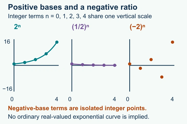In AP Calculus, the idea that the derivative of an exponential function is proportional to the function itself leads directly to the study of differential equations of the form dy/dx = ky. For positive r, the parameter k in that equation is precisely ln(r) from the geometric sequence perspective, completing the circle from discrete multiplicative change to continuous exponential growth.

Positive-base exponential curves beside isolated integer points of the alternating sequence (−2)^n. The alternating sequence is not connected as a real exponential curve. Negative-ratio geometric terms alternate at integer indices and do not define an ordinary real-valued exponential curve across every real input.

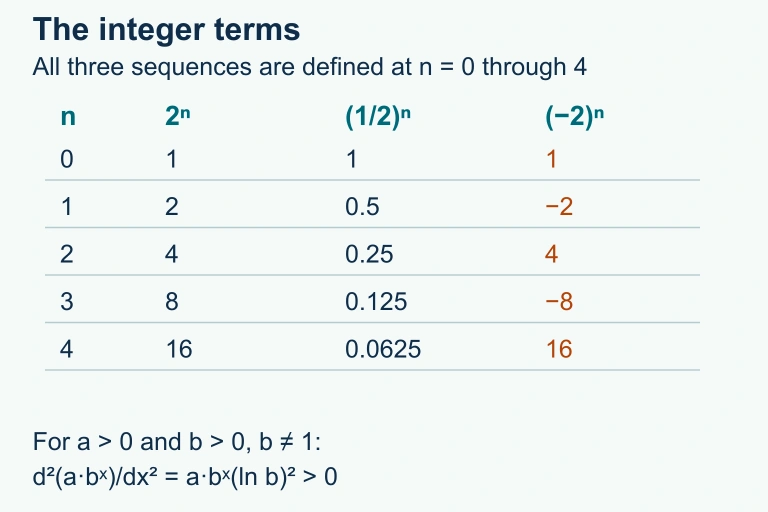Fifteen integer-index terms of three sequences, with the positive-coefficient exponential second derivative a·b^x(ln b)².

SECTION 9

Practice Problems

Question 1: CONCEPTUAL

A sequence is defined by the property that every consecutive pair of terms has the same ratio. Which of the following must be true about the sequence?

A. The first differences of the sequence are constant.
B. The sequence is arithmetic with a positive common difference.
C. The sequence is geometric, and when the logarithm of each term is taken, the resulting values form an arithmetic sequence.
D. The sequence must be increasing.
E. The sequence can be modeled by a polynomial function of degree 2.

Show answer (C)

C is correct. A constant ratio between consecutive terms defines a geometric sequence. Taking the logarithm transforms multiplicative relationships into additive ones: log(aₙ) = log(a₀) + n·log(r), which is arithmetic with common difference log(r). Choice A describes an arithmetic sequence, not geometric. Choice B incorrectly labels the sequence type. Choice D is wrong because if 0 < r < 1 or r < 0 the sequence is not necessarily increasing. Choice E is wrong because polynomial behavior requires constant higher-order differences, not constant ratios.

Question 2: BASIC CALCULATION

An arithmetic sequence has a₁ = 7 and a common difference d = −3. What is the value of a₁₅?

A. −38
B. −35
C. −32
D. 49
E. −42

Show answer (B)

B is correct. Using the explicit formula aₙ = a₁ + (n − 1)d (since the sequence is indexed from n = 1): a₁₅ = 7 + (15 − 1)(−3) = 7 + 14(−3) = 7 − 42 = −35. Choice A (−38) results from incorrectly using (n)(d) instead of (n−1)(d). Choice C (−32) would result from miscounting the number of differences. Choice D (49) results from incorrectly adding 42 instead of subtracting it. Choice E (−42) comes from computing 14(−3) and ignoring the initial term.

Question 3: INTERMEDIATE

A geometric sequence has a₂ = 18 and a₅ = 486. Find the common ratio r and the first term a₀.

A. r = 3, a₀ = 2
B. r = 3, a₀ = 6
C. r = 27, a₀ = 18/729
D. r = 9, a₀ = 2/9
E. r = 3, a₀ = 18

Show answer (A)

A is correct. From the explicit formula aₙ = a₀ · rⁿ, we get a₅/a₂ = r³. Thus r³ = 486/18 = 27, giving r = 3. Then a₂ = a₀ · 3² = 9a₀ = 18, so a₀ = 2. Choice B has a₀ = 6, which would give a₂ = 6 · 9 = 54, not 18. Choice C incorrectly treats the ratio as 27 instead of taking the cube root. Choice D squares instead of cubing. Choice E confuses a₀ with a₂.

Question 4: APPLIED

5 pts

A pharmaceutical researcher models the concentration C(n) of a drug in a patient's bloodstream, measured every hour. After the initial dose, the data collected are: n: 0 1 2 3 4 C(n): 200 150 112.5 84.375 63.28125 (a) Show that the concentration follows a geometric sequence and determine the common ratio. (b) Write an explicit formula for C(n). (c) Determine after how many whole hours the concentration first drops below 20 mg/L. (d) Explain why a linear (arithmetic) model would be inappropriate for this scenario.

Show answer

Point 1 (Geometric verification): Compute successive ratios: 150/200 = 0.75, 112.5/150 = 0.75, 84.375/112.5 = 0.75, 63.28125/84.375 = 0.75. All ratios are constant, confirming a geometric sequence with r = 0.75. Point 2 (Explicit formula): C(n) = 200 · (0.75)ⁿ, where n represents the number of hours after the dose. Point 3 (Finding the hour): Solve 200 · (0.75)ⁿ < 20, which gives (0.75)ⁿ < 0.1. Taking logarithms: n > ln(0.1)/ln(0.75) = (−2.3026)/(−0.2877) ≈ 8.004. So after 9 whole hours, the concentration first drops below 20 mg/L (since at n = 8 the concentration is approximately 20.03, and at n = 9 it is approximately 15.02). Point 4 (Why not arithmetic): An arithmetic model would subtract a fixed amount each hour. The first differences are −50, −37.5, −28.125, −21.09375, which are not constant. A linear model would eventually predict negative concentrations, which is physically impossible. The geometric model naturally approaches zero without crossing it, matching the biology of exponential drug clearance. Point 5 (Communication): Clear and correct mathematical notation throughout, with logical reasoning and justification of the sequence type using computed ratios. Five concentration bars at equally spaced hours 0 through 4: 200,150,112.5,84.375,63.28125 mg/L. Each step multiplies concentration by 0.75.

Five concentration bars at equally spaced hours 0 through 4: 200,150,112.5,84.375,63.28125 mg/L. Each step multiplies concentration by 0.75.

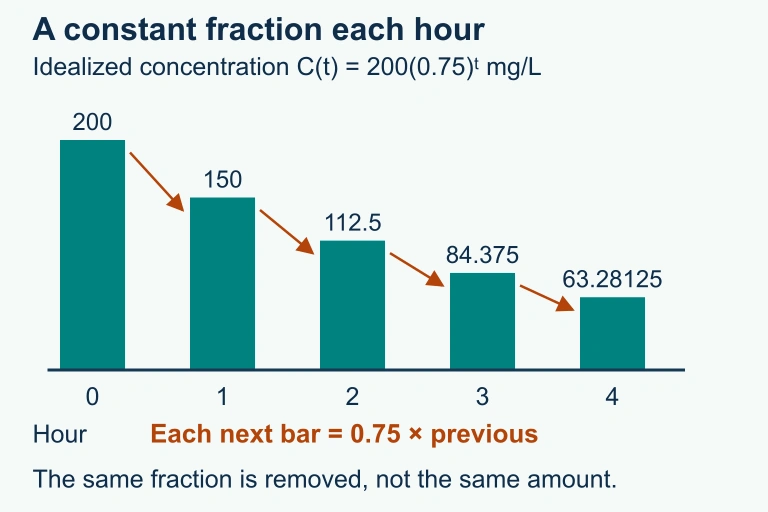A constant hourly retention factor 0.75 produces smaller absolute concentration decreases at successive equal-hour observations.

Question 5: CRITICAL THINKING

3 pts

A sequence {aₙ} satisfies the property that for all n ≥ 1, the arithmetic mean of aₙ₋₁ and aₙ₊₁ equals aₙ. (a) Prove that {aₙ} must be an arithmetic sequence. (b) A different sequence {bₙ} with all positive terms satisfies the property that for all n ≥ 1, the geometric mean of bₙ₋₁ and bₙ₊₁ equals bₙ. Prove that {bₙ} must be a geometric sequence. (c) Give an example showing that part (b) fails if the positivity condition is removed.

Show answer

Point 1 (Part a): The arithmetic mean condition gives (aₙ₋₁ + aₙ₊₁)/2 = aₙ, which rearranges to aₙ₊₁ − aₙ = aₙ − aₙ₋₁. This states that the difference between consecutive terms is constant, which is precisely the definition of an arithmetic sequence. Point 2 (Part b): The geometric mean condition (for positive terms) gives √(bₙ₋₁ · bₙ₊₁) = bₙ. Squaring both sides: bₙ₋₁ · bₙ₊₁ = bₙ². Rearranging: bₙ₊₁/bₙ = bₙ/bₙ₋₁. This shows the ratio between consecutive terms is constant, which is the definition of a geometric sequence. Point 3 (Part c): Consider the sequence bₙ = (−1)ⁿ, i.e., −1, 1, −1, 1, …. Then bₙ₋₁ · bₙ₊₁ = (−1)ⁿ⁻¹ · (−1)ⁿ⁺¹ = (−1)²ⁿ = 1 = bₙ². The geometric mean relationship holds algebraically, but the successive ratios alternate between −1 and −1, which actually is a geometric sequence with r = −1. A better counterexample: consider bₙ that alternates 2, −2, 2, −2,… Here bₙ₋₁ · bₙ₊₁ = (2)(2) = 4 = (−2)² = bₙ², but √(bₙ₋₁ · bₙ₊₁) = 2 ≠ −2 = bₙ when n is odd. So the square root (geometric mean) equals |bₙ|, not bₙ, showing the geometric mean condition as written (with the positive square root) fails to characterize the sequence properly when terms can be negative.

SUMMARY

Summary

Sequences can be classified by the nature of change between consecutive terms. An arithmetic sequence has a constant common difference d, meaning each term equals the previous term plus d, which produces constant first differences and corresponds to a linear function f(x) = a₀ + dx. A geometric sequence has a constant common ratio r, meaning each term equals the previous term times r, which produces constant successive ratios and corresponds to an exponential function g(x) = a₀ · rˣ.

To identify a sequence's type, compute both first differences and successive ratios: if the differences are constant, the model is linear; if the ratios are constant, the model is exponential. The explicit formulas aₙ = a₀ + dn and aₙ = a₀ · rⁿ allow direct computation of any term without iteration. On a semi-log plot, geometric sequences appear linear because logarithms convert multiplicative relationships into additive ones. These ideas form the conceptual bridge between discrete sequences and the continuous linear and exponential functions that are central to the AP Precalculus curriculum.