Rotational Kinematics - AP Physics C Mechanics

SECTION 1

Historical Context & Motivation

The study of rotation predates Newton, rooted in humanity's oldest scientific enterprise: astronomy. Ancient observers tracked the angular motion of celestial bodies across the sky, measuring positions in degrees along circular arcs long before anyone formalized the concept of a radian. The need to describe how quickly a wheel spins, how a planet sweeps through its orbit, or how a flywheel accelerates drove the development of rotational kinematics — the branch of mechanics that characterizes rotational motion without reference to its causes.

1609 • Kepler's Laws of Planetary Motion

Johannes Kepler published his first two laws, describing planets sweeping equal areas in equal times — an early statement relating angular displacement to time.

1687 • Newton's Principia

Isaac Newton formalized the mathematics of circular and orbital motion, connecting angular variables to the calculus he co-invented.

1736 • Euler's Mechanica

Leonhard Euler systematized rotational motion, introducing the radian as a natural measure and developing the angular analogs of linear kinematic equations.

1765 • Euler's Rigid Body Dynamics

Euler extended rotational kinematics to three dimensions, laying the groundwork for the modern treatment of angular velocity as a vector quantity.

The central question that rotational kinematics answers is deceptively simple: given an object spinning or revolving, how do we describe its position, speed, and rate of speed change at any instant? The answer mirrors linear kinematics almost perfectly — replace displacement with angle, velocity with angular velocity, and acceleration with angular acceleration — yet this elegant parallel conceals subtleties that the AP Physics C exam loves to probe.

SECTION 2

Core Principles & Definitions

Rotational kinematics is built on three angular variables that serve as direct analogs to their linear counterparts. Understanding these variables and the sign conventions attached to them is essential before tackling any problem involving spinning objects.

Angular Displacement (θ)

The angle through which an object rotates, measured in radians. One full revolution equals 2π rad. Unlike degrees, radians are dimensionless ratios (arc length / radius), making them natural for calculus operations.

Angular Velocity (ω)

The rate of change of angular displacement: ω = dθ/dt, measured in rad/s. By convention, counterclockwise (CCW) is positive when viewed from the standard orientation. Angular velocity is an axial vector directed along the rotation axis via the right-hand rule.

Angular Acceleration (α)

The rate of change of angular velocity: α = dω/dt = d²θ/dt², measured in rad/s². When α and ω share the same sign, the object speeds up; when they differ, the object slows down.

The Linear–Angular Bridge

Every point on a rigid body at distance r from the axis satisfies s = rθ, v_t = rω, and a_t = rα. These bridge equations connect rotational kinematics to the tangential linear quantities the AP exam frequently tests.

SECTION 3

Visualizing Rotational Variables

A point P on a spinning disk at radius r from the axis traces a circular path. The angular displacement θ (cyan arc) defines the rotation, while the tangential velocity v = rω (violet arrow) is always perpendicular to the radius. The tangential acceleration a_t = rα (pink) acts along the velocity direction, and the centripetal acceleration a_c = ω²r (amber, dashed) points inward toward the axis.

The diagram above captures the essential geometry of rotational kinematics for a rigid body. Every point on the body shares the same values of θ, ω, and α at any instant — that is what makes these variables so powerful for describing rigid-body rotation. However, the linear quantities differ by radius: a point twice as far from the axis moves with twice the tangential speed. This r-dependence is precisely encoded in the bridge equations s = rθ, v_t = rω, and a_t = rα. Note also the centripetal acceleration a_c = ω²r, which exists even at constant angular velocity and always points radially inward.

SECTION 4

Mathematical Framework

Fundamental Definitions (Calculus Form)

ANGULAR VELOCITY

ω = dθ / dt

ω is the instantaneous angular velocity in rad/s; θ is the angular position in radians; t is time in seconds.

ANGULAR ACCELERATION

α = dω / dt = d²θ / dt²

α is the instantaneous angular acceleration in rad/s². When α is constant, the rotational kinematic equations below apply directly.

Constant Angular Acceleration Equations

When α is constant, we integrate the definitions above to obtain four kinematic equations that mirror their linear counterparts exactly. The AP Physics C exam expects you to derive these from calculus and to apply them fluently.

EQUATION 1

ω = ω₀ + αt

Analogous to v = v₀ + at. Gives final angular velocity as a function of time.

EQUATION 2

θ = θ₀ + ω₀t + ½αt²

Analogous to x = x₀ + v₀t + ½at². Gives angular position as a function of time.

EQUATION 3

ω² = ω₀² + 2α(θ − θ₀)

Analogous to v² = v₀² + 2a(x − x₀). Eliminates time from the relationship.

EQUATION 4

θ − θ₀ = ½(ω₀ + ω)t

The average angular velocity form. Useful when α is not explicitly needed.

Bridge Equations (Linear ↔ Angular)

LINEAR–ANGULAR BRIDGE

s = rθ v_t = rω a_t = rα a_c = ω²r = v²/r

These hold for any point at distance r from the rotation axis of a rigid body. The tangential acceleration a_t changes the speed; the centripetal acceleration a_c changes the direction.

ℹ

Calculus Note

A blue motor drives a gold flywheel through a continuous horizontal shaft with two bearings. A fixed brake caliper contacts the wheel rim inside a partial protective guard. A flywheel subject to viscous drag slows with angular acceleration proportional to −ω. This exponential model uses a different torque law from a dry-friction brake.

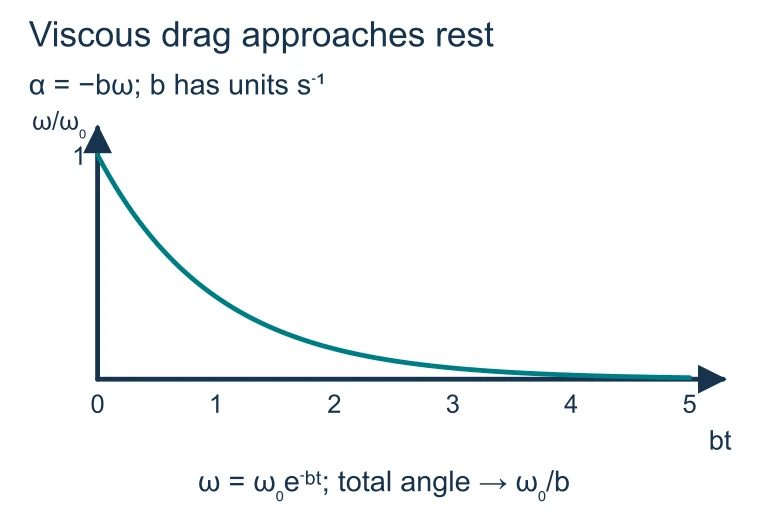Exponential angular-speed decay. For α = −bω with b measured in s⁻¹, angular speed is ω₀e⁻ᵇᵗ. It approaches zero asymptotically while total angular displacement approaches ω₀/b. For α = −bω with b measured in s⁻¹, angular speed is ω₀e⁻ᵇᵗ. It approaches zero asymptotically while total angular displacement approaches ω₀/b.

SECTION 5

Linear–Angular Analogy Table

One of the most powerful study strategies for rotational kinematics is to internalize the systematic correspondence between linear and angular quantities. The table below organizes this analogy comprehensively, serving as a reference you can mentally reconstruct during the exam.

Linear Quantity	Symbol	Angular Quantity	Symbol
Displacement	x, s	Angular displacement	θ
Velocity	v	Angular velocity	ω
Acceleration	a	Angular acceleration	α
Mass	m	Moment of inertia	I
Force	F	Torque	τ
Kinetic energy ½mv²	K	Rotational KE ½Iω²	K_rot
Momentum mv	p	Angular momentum Iω	L

Systematic correspondence between linear and rotational quantities

For constant angular acceleration α = 2 rad/s² and initial angular velocity ω₀ = 1 rad/s, the ω-vs-t graph is a straight line with slope α. The area under the ω–t curve equals the angular displacement Δθ, just as the area under a v–t curve equals linear displacement.

The graphical interpretation of rotational kinematics is identical to its linear counterpart and is a frequent subject of AP exam questions. On an ω–t graph, the slope at any point gives the instantaneous angular acceleration α, while the area between the curve and the time axis over an interval gives the angular displacement Δθ during that interval. Likewise, on an α–t graph, the area under the curve yields the change in angular velocity Δω. Recognizing these graphical relationships allows you to extract quantitative information even when an algebraic expression for α(t) is unavailable — you simply estimate or compute the area geometrically.

SECTION 6

Worked Example

A centrifuge rotor starts from rest and accelerates uniformly at α = 150 rad/s² for 8.0 s, then spins at constant angular velocity for 60 s, and finally decelerates uniformly to rest over 12.0 s. Find (a) the maximum angular velocity, (b) the total angular displacement, and (c) the tangential speed of a point 0.10 m from the axis at maximum ω.

Worked example

1
Step 1 — Find maximum angular velocity

During the acceleration phase, ω₀ = 0, α = 150 rad/s², t₁ = 8.0 s. Using ω = ω₀ + αt: ω_max = 0 + (150)(8.0) = 1200 rad/s.

ω_max = 1200 rad/s ≈ 11 460 rpm
2
Step 2 — Angular displacement during acceleration

θ₁ = ω₀t + ½αt² = 0 + ½(150)(8.0)² = ½(150)(64) = 4800 rad.

θ₁ = 4800 rad
3
Step 3 — Angular displacement at constant ω

During the constant-velocity phase, α = 0 and t₂ = 60 s. θ₂ = ω_max × t₂ = 1200 × 60 = 72 000 rad.

θ₂ = 72 000 rad
4
Step 4 — Angular displacement during deceleration

The rotor decelerates from 1200 rad/s to 0 over t₃ = 12.0 s. Using θ = ½(ω₀ + ω)t: θ₃ = ½(1200 + 0)(12.0) = 7200 rad.

θ₃ = 7200 rad
5
Step 5 — Total displacement and tangential speed

Total angular displacement: θ_total = 4800 + 72 000 + 7200 = 84 000 rad. In revolutions: 84 000 / (2π) ≈ 13 370 rev. The tangential speed at r = 0.10 m when ω = 1200 rad/s is v_t = rω = (0.10)(1200) = 120 m/s.

θ_total = 84 000 rad ≈ 13 370 rev; $v_t$ = 120 m/s

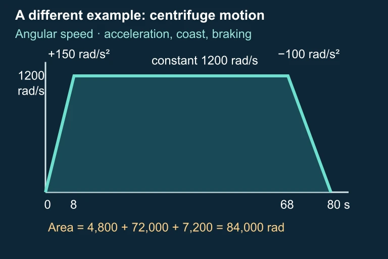Separate centrifuge acceleration, coast and braking example.

SECTION 7

Common Pitfalls & Exam Tips

Common Pitfall	Why It's Wrong	Correct Approach
Using degrees in kinematic equations	The equations ω = dθ/dt and s = rθ only work when θ is in radians. Mixing in degrees produces answers off by a factor of π/180.	Always convert to radians first. 1 rev = 2π rad; 1° = π/180 rad.
Forgetting centripetal acceleration	Even at constant ω, a point on a rotating body has centripetal acceleration $a_c$ = ω²r directed inward.	The total linear acceleration is the vector sum of $a_t$ and $a_c$ . Compute \|a\| = √( $a_t$ ² + $a_c$ ²).
Applying constant-α equations when α varies	If α depends on t or θ, the four standard kinematic equations are invalid.	Integrate directly: ω = ∫α dt, θ = ∫ω dt. Watch for variable-separable forms.
Sign errors with deceleration	If ω is positive but the object slows down, α must be negative. Students often enter a positive α for both phases.	Define a positive direction first. If ω > 0 and the object decelerates, set α < 0.

Key pitfalls tested on AP Physics C: Mechanics exams

★

Key takeaway

EXAM STRATEGY

SECTION 8

Connection to Rotational Dynamics & Beyond

Rotational kinematics describes how objects rotate; rotational dynamics explains why. Once you know α from kinematics, Newton's second law for rotation — τ_net = Iα — connects that angular acceleration to the net torque and the moment of inertia. The table below maps the kinematic concepts you've learned to their dynamic extensions, previewing where this unit is headed.

Kinematics (this lesson)	Dynamics (next topics)
α = dω/dt (describes motion)	τ_net = Iα (explains cause of motion)
ω and θ as functions of t	Work–energy theorem: W = ∫τ dθ = ΔK_rot
Constant-α equations	Rolling without slipping: v_cm = Rω, a_cm = Rα
Bridge equations (v = rω)	Angular momentum: L = Iω, conservation of L

From kinematics to dynamics: what comes next

For non-constant angular acceleration, AP Physics C frequently presents torque as a function of angle (τ(θ)) or time (τ(t)). In these cases you must combine the dynamic equation α = τ/I with integration to recover ω(t) and θ(t). The mathematical fluency you develop in this kinematics lesson — particularly comfort with integrating α(t) — directly transfers to those more complex problems. Additionally, the bridge equations resurface in rolling-without-slipping problems, where the constraint v_cm = Rω links translational and rotational motion of a single object.

SECTION 9

Practice Problems

Question 1: CONCEPTUAL

A wheel rotates with constant angular velocity ω. Which statement about a point on the rim is correct? A) Its tangential acceleration is zero and its centripetal acceleration is zero. B) Its tangential acceleration is nonzero and its centripetal acceleration is zero. C) Its tangential acceleration is zero and its centripetal acceleration is nonzero. D) Both its tangential and centripetal accelerations are nonzero.

A. Its tangential acceleration is zero and its centripetal acceleration is zero.
B. Its tangential acceleration is nonzero and its centripetal acceleration is zero.
C. Its tangential acceleration is zero and its centripetal acceleration is nonzero.
D. Both its tangential and centripetal accelerations are nonzero.

Show answer (C)

The correct answer is C. When ω is constant, α = 0, so the tangential acceleration a_t = rα = 0. However, the point is still moving in a circle, so it must have centripetal acceleration a_c = ω²r ≠ 0 directed toward the center. Option A incorrectly claims centripetal acceleration is zero — uniform circular motion still requires centripetal acceleration. Option B reverses the situation: with constant ω, there is no tangential acceleration. Option D is incorrect because a_t = 0 when angular velocity is constant.

Question 2: BASIC CALCULATION

A turbine blade accelerates uniformly from rest to 3000 rpm in 10 s. What is the angular acceleration α? A) 300 rad/s² B) 100π rad/s² ≈ 314 rad/s² C) 10π rad/s² ≈ 31.4 rad/s² D) 50π rad/s² ≈ 157 rad/s²

A. 300 rad/s²
B. 100π rad/s² ≈ 314 rad/s²
C. 10π rad/s² ≈ 31.4 rad/s²
D. 50π rad/s² ≈ 157 rad/s²

Show answer (C)

The correct answer is C. First convert 3000 rpm to rad/s: ω = 3000 × (2π/60) = 100π rad/s. Then α = (ω − ω₀)/t = (100π − 0)/10 = 10π ≈ 31.4 rad/s². Option A results from failing to convert rpm to rad/s (using 3000/10 = 300). Option B uses α = ω/t but with an incorrect t or conversion. Option D results from dividing by 2 instead of 10, or a miscalculation in the conversion step.

Question 3: INTERMEDIATE

A disk has angular acceleration α(t) = 6t (rad/s²), starting from rest at t = 0. What is the angular displacement θ at t = 2 s? A) 4 rad B) 8 rad C) 12 rad D) 24 rad

A. 4 rad
B. 8 rad
C. 12 rad
D. 24 rad

Show answer (B)

The correct answer is B. Since α is not constant, we must integrate. ω(t) = ∫₀ᵗ 6t′ dt′ = 3t². Then θ(t) = ∫₀ᵗ 3t′² dt′ = t³. At t = 2 s: θ = (2)³ = 8 rad. Option A (4 rad) may result from computing ω(2) = 3(4) = 12 and then incorrectly halving. Option C (12 rad) is ω(2) = 12, not θ. Option D (24 rad) results from incorrectly using θ = ½αt² with α(2) = 12, yielding ½(12)(4) = 24, which is wrong because α is not constant.

Question 4: APPLIED

A grinding wheel of radius R = 0.20 m starts from rest and accelerates uniformly at α = 5.0 rad/s² for 4.0 s, then rotates at constant angular velocity. (a) Derive an expression for ω(t) during the acceleration phase and evaluate it at t = 4.0 s. (b) Find the total angle turned through during the first 4.0 s. (c) Calculate the tangential speed, centripetal acceleration, and total linear acceleration of a point on the rim at t = 4.0 s. (d) After the wheel reaches constant ω, a brake is applied producing a constant angular deceleration that brings the wheel to rest after 10 additional revolutions. Find the angular deceleration.

Show answer

(a) During the acceleration phase with constant α, integrating α = dω/dt from rest gives ω(t) = αt = 5.0t. At t = 4.0 s: ω = 5.0 × 4.0 = 20 rad/s. [1 pt] (b) θ = ω₀t + ½αt² = 0 + ½(5.0)(4.0)² = 40 rad. [1 pt] (c) At t = 4.0 s, ω = 20 rad/s and α = 5.0 rad/s² still applies (instant just as acceleration ends): • v_t = Rω = (0.20)(20) = 4.0 m/s [1 pt] • a_c = ω²R = (20)²(0.20) = 80 m/s² [1 pt] • a_t = Rα = (0.20)(5.0) = 1.0 m/s²; total |a| = √(1.0² + 80²) ≈ 80 m/s² [1 pt] (d) The wheel starts the braking phase at ω₀ = 20 rad/s and stops after Δθ = 10 rev = 20π rad. Using ω² = ω₀² + 2αΔθ with ω = 0: [1 pt setup] 0 = 400 + 2α(20π) → α = −400/(40π) = −10/π ≈ −3.18 rad/s². [1 pt]

Question 5: CRITICAL THINKING

A shaft has angular acceleration α = −bω, where b is a positive constant and ω is the angular velocity. At t = 0, the shaft has angular velocity ω₀. (a) Solve the differential equation to find ω(t). (b) Find θ(t) and determine the total angle turned through as t → ∞. (c) Explain physically why the shaft never actually stops in finite time, and identify the type of motion this represents.

Show answer

(a) The equation dω/dt = −bω is a first-order separable ODE. Separating: dω/ω = −b dt. Integrating: ln(ω) = −bt + C. With ω(0) = ω₀: ω(t) = ω₀

e^{−bt}

. [1 pt] (b) θ(t) = ∫₀ᵗ ω₀e^(−bt′) dt′ = (ω₀/b)[1 −

e^{−bt}

]. As t → ∞,

e^{−bt}

→ 0, so θ_total = ω₀/b. [1 pt for θ(t), 1 pt for limit] (c) This is exponential decay of angular velocity, analogous to a velocity-dependent drag force. Because the decelerating mechanism (α = −bω) weakens in proportion to the speed itself, the shaft asymptotically approaches rest. At any finite time, ω is still positive (though potentially negligibly small). This mirrors a first-order RC discharge or viscous drag in a fluid. [1 pt]