Resistive Forces - AP Physics C Mechanics

SECTION 1

Historical Context & Motivation

For centuries, the study of motion was entangled with the effects of resistive forces — forces that oppose the relative motion of an object through a medium or across a surface. Aristotle believed that a constant force was necessary to maintain constant velocity, an intuition shaped entirely by the ubiquity of friction and air resistance in everyday experience. It was not until the scientific revolution that thinkers began to disentangle the idealized laws of motion from the ever-present dissipative effects of resistive forces. Understanding how to model these forces quantitatively has been essential to fields ranging from ballistics and aeronautics to automotive engineering and biomechanics.

1687 • Newton's Principia

Isaac Newton published the Principia, formulating the laws of motion and proposing that fluid resistance is proportional to velocity for slow flows and to velocity squared for fast flows.

1851 • Stokes' Law

George Gabriel Stokes derived the drag force on a small sphere moving through a viscous fluid at low Reynolds number: F = 6πηrv, providing the first rigorous linear drag model.

1883 • Reynolds Number

Osborne Reynolds introduced the dimensionless ratio that predicts the transition from laminar (linear drag) to turbulent (quadratic drag) flow, unifying the two regimes Newton had identified.

1920s • Modern Aerodynamics

Ludwig Prandtl and his students developed boundary-layer theory, enabling engineers to compute drag coefficients for streamlined bodies and laying the foundation for modern aeronautical design.

The central question this lesson addresses is deceptively simple: how do we incorporate velocity-dependent resistive forces into Newton's second law, and what new mathematical behaviors arise as a result? Unlike constant forces such as gravity near Earth's surface, resistive forces depend on the speed of the object, which means that the resulting differential equations are often nonlinear and produce phenomena like terminal velocity that have no analogue in the constant-force world.

SECTION 2

Core Principles & Definitions

Resistive forces encompass any force that opposes the relative motion of an object. In the AP Physics C: Mechanics framework, the two most important categories are surface friction (kinetic and static) and fluid drag. While kinetic friction is typically modeled as velocity-independent (f_k = μ_kN), fluid resistance introduces a fundamentally different character: the resistive force depends on the object's speed, making the equation of motion a differential equation whose solution yields exponential approach to a limiting velocity.

Linear Drag (f = −bv)

Dominates at low speeds and small length scales (low Reynolds number). The drag force is directly proportional to velocity. Common in viscous flows around small particles and in introductory AP problems.

Quadratic Drag (f = −cv²)

Dominates at high speeds and large length scales (high Reynolds number). The drag force scales with the square of velocity. Relevant for falling skydivers, automobiles, and projectiles in air.

Terminal Velocity

The constant speed reached when the net force on a falling object becomes zero because the drag force equals the gravitational force. The object's acceleration vanishes and velocity remains constant thereafter.

Time Constant (τ = m/b)

For linear drag, τ characterizes how quickly the object approaches terminal velocity. After one time constant, the velocity reaches approximately 63% of its terminal value — a hallmark of exponential behavior.

✦

KEY TAKEAWAY

Think of a resistive force as a thermostat for velocity. Just as a thermostat increases its corrective action when the room temperature deviates further from the setpoint, a velocity-dependent drag force pushes back harder the faster an object moves. The system self-regulates until it reaches equilibrium — the terminal velocity — where driving and resistive forces exactly balance.

SECTION 3

Visual Explanation — Free-Body Diagram with Drag

A falling object of mass m experiences its weight mg directed downward (red) and a linear drag force bv directed upward (green), opposing the velocity (amber). When these forces balance, the acceleration is zero and the object has reached terminal velocity.

The diagram above illustrates the essential physics of an object falling through a resistive medium. Taking the downward direction as positive, the gravitational force mg accelerates the object, while the drag force bv retards it. Early in the fall, when v is small, the drag is negligible and the object accelerates at nearly g. As the object speeds up, the drag force grows until it equals mg, at which point the net force is zero and the velocity plateaus at the terminal velocity v_t = mg/b.

SECTION 4

Mathematical Framework

Linear Drag: Deriving v(t) for a Falling Object

Consider an object of mass m released from rest and falling through a fluid that exerts a linear drag force. Choosing the downward direction as positive, Newton's second law gives the first-order linear ODE:

EQUATION OF MOTION (LINEAR DRAG)

m(dv/dt) = mg − bv

where b is the drag coefficient (units: kg/s), v is the instantaneous speed, and g is the gravitational acceleration.

To solve, separate variables. Rearranging: dv/(mg − bv) = dt/m. Integrating both sides with the initial condition v(0) = 0 and defining the terminal velocity v_t = mg/b and the time constant τ = m/b, we obtain:

VELOCITY AS A FUNCTION OF TIME

v(t) = v_t (1 − e^(−t/τ))

v_t = mg/b (terminal velocity), τ = m/b (time constant). As t → ∞, v → v_t exponentially.

The acceleration can be found by differentiating: a(t) = (v_t/τ) e^−t/τ = g e^−t/τ. At t = 0 the acceleration equals g, confirming that the object initially behaves as if in free fall. The acceleration then decays exponentially to zero as the object asymptotically approaches terminal velocity.

Quadratic Drag

EQUATION OF MOTION (QUADRATIC DRAG)

m(dv/dt) = mg − ½CρAv²

C = drag coefficient (dimensionless), ρ = fluid density, A = cross-sectional area. The terminal velocity is v_t = √(2mg / CρA).

For quadratic drag, separation of variables yields an integral involving partial fractions (or equivalently, inverse hyperbolic tangent). The solution for an object released from rest falling vertically is v(t) = v_t tanh(gt/v_t). While the AP exam most frequently tests the linear drag model, you should recognize the quadratic form and be comfortable setting the net force to zero to find terminal velocity in either regime.

POSITION AS A FUNCTION OF TIME (LINEAR DRAG)

x(t) = v_t [ t − τ(1 − e^(−t/τ)) ]

Obtained by integrating v(t). As t → ∞, the position grows linearly (constant velocity v_t) with a constant offset −v_tτ.

SECTION 5

Velocity vs. Time: Comparing Drag Regimes

Comparison of velocity versus time for three scenarios: no drag (purple, linear increase), linear drag (cyan, exponential approach), and quadratic drag (pink, hyperbolic tangent approach). Both drag curves asymptotically approach the terminal velocity v_t (amber dashed line). At t = τ the linear drag curve reaches 63% of v_t.

The graph above makes several important features visible. Without drag, velocity increases without bound at a constant rate g. With either linear or quadratic drag, the velocity curve bends over and approaches terminal velocity asymptotically. Notice that the quadratic drag curve initially follows the no-drag line more closely (because at small v, the v² term is very small), but it catches up and ultimately approaches the same terminal speed. The slope of each curve at any point equals the instantaneous acceleration, which is always less than g and decreases monotonically to zero.

💡

AP EXAM TIP

When the AP exam asks you to sketch v(t) or a(t) for an object falling with drag, remember three checkpoints: (1) at t = 0, v = 0 and a = g; (2) the curve is concave down (a is decreasing); (3) as t → ∞, v → v_t and a → 0. These three features earn full credit on most FRQ sketch prompts.

One bead is immersed away from vessel walls below the free surface; circular magnifier depicts the same bead. Flow texture is uncalibrated; buoyancy/wall effects are excluded in the declared ideal model. Separate exact panel: A computed velocity curve rises from zero toward a dashed4.9m/s asymptote; downward-positive linear drag model is shown. A bead released from rest accelerates until upward drag balances its weight in the model. Linear and quadratic drag give different equations and approach curves, with coefficients and conditions specified separately.

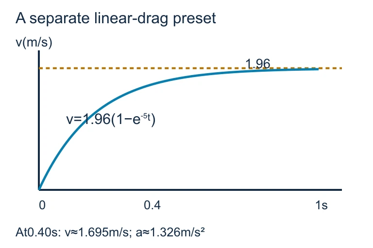A linear-drag example. For v = 1.96(1 − e⁻⁵ᵗ) m/s, the terminal speed is 1.96 m/s. At t = 0.40 s, v ≈ 1.695 m/s and acceleration is about 1.326 m/s². For v = 1.96(1 − e⁻⁵ᵗ) m/s, the terminal speed is 1.96 m/s. At t = 0.40 s, v ≈ 1.695 m/s and acceleration is about 1.326 m/s².

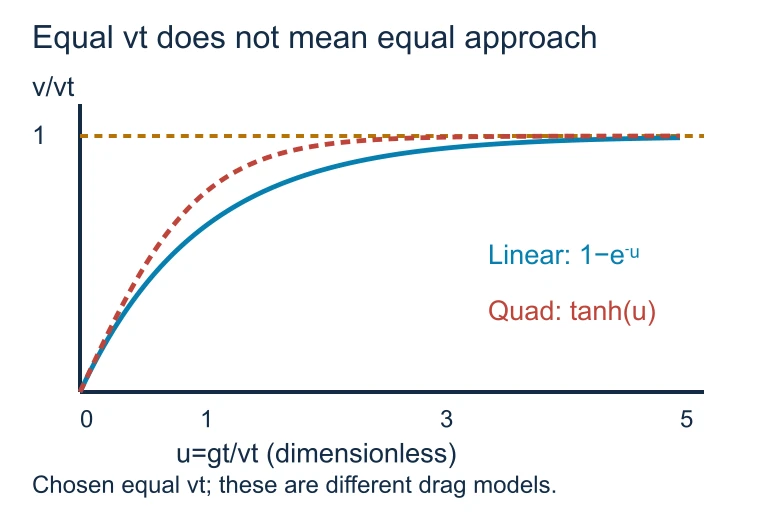Comparing drag laws. Choose coefficients so the two models share terminal speed vₜ and define u = gt/vₜ. The linear-drag curve is v/vₜ = 1 − e⁻ᵘ; the quadratic-drag curve is tanh(u). Choose coefficients so the two models share terminal speed vₜ and define u = gt/vₜ. The linear-drag curve is v/vₜ = 1 − e⁻ᵘ; the quadratic-drag curve is tanh(u).

SECTION 6

Worked Example — Falling Sphere with Linear Drag

A steel ball of mass 0.050 kg is released from rest in a tank of oil. The linear drag coefficient is b = 0.25 kg/s. Find (a) the terminal velocity, (b) the time constant, (c) the velocity at t = 0.40 s, and (d) the acceleration at t = 0.40 s.

Steel Ball Falling in Oil

1
Step 1 — Identify Given Values

Mass: m = 0.050 kg. Drag coefficient: b = 0.25 kg/s. Initial velocity: v₀ = 0. Gravitational acceleration: g = 9.8 m/s².
2
Step 2 — Terminal Velocity

At terminal velocity, the net force is zero: mg = bv_t. Therefore v_t = mg/b = (0.050)(9.8) / 0.25 = 0.49 / 0.25.

$v_t$ = 1.96 m/s
3
Step 3 — Time Constant

τ = m/b = 0.050 / 0.25.

τ = 0.20 s
4
Step 4 — Velocity at t = 0.40 s

Using v(t) = v_t(1 − e^−t/τ): v(0.40) = 1.96(1 − e^−0.40/0.20) = 1.96(1 − e⁻²) = 1.96(1 − 0.1353) = 1.96 × 0.8647.

v(0.40 s) ≈ 1.69 m/s
5
Step 5 — Acceleration at t = 0.40 s

a(t) = g e^−t/τ = 9.8 × e⁻² = 9.8 × 0.1353.

a(0.40 s) ≈ 1.33 m/s²

Notice that at t = 2τ the ball has already reached about 86.5% of terminal velocity, and the acceleration has dropped to about 13.5% of g. This rapid convergence is characteristic of exponential decay — after just five time constants, the velocity is within 1% of v_t.

SECTION 7

Linear vs. Quadratic Drag — When to Use Each

Feature	Linear Drag (f = bv)	Quadratic Drag (f = ½CρAv²)
Reynolds Number	Re ≪ 1 (creeping / Stokes flow)	Re ≫ 1 (turbulent flow)
Typical Situations	Small particles in viscous fluids, fog droplets, pollen grains	Baseballs, cars, skydivers, bullets in air
Terminal Velocity	$v_t$ = mg / b	$v_t$ = √(2mg / CρA)
v(t) Solution	$v_t$ (1 − $e^{−t/τ}$ )	$v_t$ tanh(gt / $v_t$ )
ODE Type	First-order linear — separable and integrable in closed form	First-order nonlinear — separable, requires partial fractions
AP Exam Emphasis	Frequently tested; expect full derivations and graphical analysis	Setting up the equation and finding $v_t$ ; full solution rarely required

Key differences between linear and quadratic drag models.

✦

KEY TAKEAWAY

Choosing the correct drag model is analogous to choosing the right tool in engineering: a wrench and a screwdriver both tighten fasteners, but applying the wrong one wastes effort and gives poor results. In the same way, applying linear drag to a skydiver (where quadratic drag dominates) would yield a wildly incorrect terminal velocity. The Reynolds number serves as your diagnostic — low Re calls for linear drag, high Re calls for quadratic.

SECTION 8

Connection to Advanced Theory

The differential equations encountered in this lesson are prototypes for much deeper ideas in physics and mathematics. The linear drag ODE, m(dv/dt) + bv = mg, is a first-order linear ODE with constant coefficients — the same mathematical structure that governs RC circuits in electromagnetism, radioactive decay in nuclear physics, and Newton's law of cooling in thermodynamics. The time constant τ = m/b is directly analogous to τ = RC in a charging capacitor.

AP Mechanics Concept	Advanced / Cross-disciplinary Analogue
Linear drag ODE: m dv/dt + bv = mg	RC circuit: R dq/dt + q/C = ε (E&M)
Terminal velocity as steady-state	Steady-state current in RL circuits; chemical equilibrium in kinetics
Quadratic drag (nonlinear ODE)	Navier–Stokes equations (fluid dynamics); logistic growth (biology)
Exponential approach to equilibrium	Damped oscillations (mechanics); signal attenuation (signal processing)

Parallels between resistive force dynamics and advanced topics.

In more advanced treatments, resistive forces in two dimensions produce coupled differential equations. For a projectile launched at an angle through a medium with quadratic drag, the equations of motion cannot generally be solved in closed form and require numerical methods — a topic explored in computational physics. The AP exam, however, restricts itself to one-dimensional scenarios and linear drag, so mastering the exponential solution is the essential goal.

SECTION 9

Practice Problems

Question 1: CONCEPTUAL

An object falls from rest through a fluid that exerts a linear drag force f = bv. Which of the following best describes how the object's acceleration changes as a function of time?

A. The acceleration remains constant at g throughout the fall.
B. The acceleration starts at g and decreases linearly to zero.
C. The acceleration starts at g and decreases exponentially toward zero.
D. The acceleration starts at zero and increases exponentially toward g.

Show answer (C)

The correct answer is C. From Newton's second law with linear drag: a(t) = g

e^{−t/τ}

. At t = 0, a = g, and a decays exponentially to zero as the object approaches terminal velocity. Choice A is wrong because it ignores drag entirely. Choice B is wrong because the decrease is exponential, not linear — the rate of change of acceleration is proportional to the acceleration itself. Choice D is wrong because it reverses the behavior: the object starts with maximum acceleration, not zero.

Question 2: BASIC CALCULATION

A 2.0 kg object falls through a medium with linear drag coefficient b = 4.0 kg/s. What is the terminal velocity of the object? (Use g = 10 m/s².)

A. 0.50 m/s
B. 2.0 m/s
C. 5.0 m/s
D. 20 m/s

Show answer (C)

The correct answer is C. At terminal velocity, mg = bv_t, so

v_t

= mg/b = (2.0)(10)/4.0 = 5.0 m/s. Choice A (0.50 m/s) results from computing b/mg instead of mg/b. Choice B (2.0 m/s) equals the mass, which is not the correct expression. Choice D (20 m/s) results from computing mg without dividing by b.

Question 3: INTERMEDIATE

A 0.50 kg object is released from rest in a fluid with linear drag coefficient b = 2.5 kg/s. How long after release does the object reach 95% of its terminal velocity? (Use g = 10 m/s².)

A. 0.20 s
B. 0.40 s
C. 0.60 s
D. 1.0 s

Show answer (C)

The correct answer is C. The time constant is τ = m/b = 0.50/2.5 = 0.20 s. The velocity is v(t) =

v_t

(1 −

e^{−t/τ}

). Setting v/

v_t

= 0.95 gives 1 −

e^{−t/τ}

= 0.95, so

e^{−t/τ}

= 0.05, and −t/τ = ln(0.05) ≈ −3.0. Therefore t ≈ 3.0τ = 3.0 × 0.20 = 0.60 s. Choice A equals one time constant (63% of

v_t

, not 95%). Choice B equals two time constants (86.5% of

v_t

). Choice D equals five time constants (99.3%), which overshoots the target.

Question 4: APPLIED

4 pts

A small sphere of mass m is projected vertically upward with initial speed v₀ through a medium that exerts a linear drag force f = −bv (opposing the velocity at all times). (a) Write the differential equation governing the sphere's velocity during the upward portion of its motion. Take upward as positive. (1 point) (b) Solve the differential equation to find v(t) during the upward portion. (1 point) (c) Find the time t_up at which the sphere momentarily stops. (1 point) (d) Explain qualitatively why the time to reach maximum height is less than v₀/g. (1 point)

Show answer

Rubric breakdown: (a) [1 point] During upward motion (v > 0), both gravity and drag act downward (negative). Newton's second law: m(dv/dt) = −mg − bv. (b) [1 point] Rewrite as dv/dt = −g − (b/m)v. This is a first-order linear ODE. Separating variables: dv/(g + (b/m)v) = −dt. Integrating with v(0) = v₀ gives v(t) = −(mg/b) + (v₀ + mg/b)

e^{−bt/m}

. Equivalently, v(t) = (v₀ +

v_t

)

e^{−t/τ}

−

v_t

, where

v_t

= mg/b and τ = m/b. (c) [1 point] Setting v(t_up) = 0: (v₀ +

v_t

)

e^{−t_up/τ}

v_t

. Solving: t_up = τ ln(1 + v₀/

v_t

) = (m/b) ln(1 + bv₀/(mg)). (d) [1 point] During the upward journey, both gravity and drag decelerate the sphere, so the net deceleration is greater than g at every instant. This means the sphere slows to rest faster than it would in the absence of drag, making t_up < v₀/g.

Question 5: CRITICAL THINKING

5 pts

A researcher drops identical steel spheres (mass m = 0.10 kg) from rest in a tall cylinder of glycerin and records the velocity as a function of time. The data suggest linear drag is appropriate. The measured terminal velocity is

v_t

= 0.40 m/s. Use g = 10 m/s². (a) Determine the drag coefficient b. (1 point) (b) Write an expression for the position y(t) of the sphere, taking the release point as y = 0 and downward as positive. (1 point) (c) Find the distance fallen during the first time constant τ. Express your answer both symbolically and numerically. (1 point) (d) On a clearly labeled set of axes, sketch graphs of v(t), a(t), and y(t) for 0 ≤ t ≤ 5τ. Identify key features (initial slopes, asymptotic values, concavity). (1 point) (e) The researcher now uses a sphere of mass 2m in the same glycerin. Assuming the drag coefficient b remains the same, determine the new terminal velocity and the new time constant. Explain physically why the heavier sphere takes longer to approach terminal velocity. (1 point)

Show answer

Rubric breakdown: (a) [1 point]

v_t

= mg/b → b = mg/

v_t

= (0.10)(10)/0.40 = 2.5 kg/s. (b) [1 point] y(t) =

v_t

[t − τ(1 −

e^{−t/τ}

)], where τ = m/b = 0.10/2.5 = 0.040 s. This is obtained by integrating v(t) =

v_t

(1 −

e^{−t/τ}

) with y(0) = 0. (c) [1 point] At t = τ: y(τ) =

v_t

[τ − τ(1 −

e^{−1}

)] =

v_t

e^{−1}

v_t

τ / e. Numerically: y(τ) = (0.40)(0.040)/e = 0.016/2.718 ≈ 0.0059 m ≈ 5.9 mm. (d) [1 point] v(t): starts at 0, increases with initial slope g = 10 m/s², concave down, asymptotically approaches

v_t

= 0.40 m/s. a(t): starts at g = 10 m/s², decreases exponentially (concave up from below), approaches 0. y(t): starts at 0, initially parabolic (like ½gt² for small t), becomes linear with slope

v_t

for large t. All three curves must have correct initial values, correct asymptotic behavior, and correct concavity. (e) [1 point] New terminal velocity:

v_t

' = (2m)g/b = 2(mg/b) = 2 × 0.40 = 0.80 m/s. New time constant: τ' = 2m/b = 2 × 0.040 = 0.080 s. The heavier sphere takes longer (larger τ) because it has more inertia — for a given velocity, the drag force is the same, but the deceleration (F/m) the drag produces is half as large, so the velocity takes longer to saturate.

SUMMARY

Lesson Summary

Summary

Resistive forces oppose an object's motion through a medium and are typically velocity-dependent. For AP Physics C: Mechanics, the most important model is linear drag (f = bv), which leads to the first-order linear ODE m(dv/dt) = mg − bv. Solving with the initial condition v(0) = 0 yields v(t) = $v_t$ (1 − $e^{−t/τ}$ ), where the terminal velocity is $v_t$ = mg/b and the time constant is τ = m/b. The acceleration decays exponentially from g to zero: a(t) = g $e^{−t/τ}$ .

For objects at higher speeds in less viscous media, quadratic drag (f = ½CρAv²) is more appropriate, yielding $v_t$ = √(2mg/CρA) and a hyperbolic tangent solution. On the AP exam, you should be able to set up Newton's second law with drag, solve the linear ODE by separation of variables, find terminal velocity in either regime, and sketch or interpret v(t), a(t), and y(t) graphs. The mathematical structure — exponential approach to a steady state governed by a time constant — recurs throughout physics, from RC circuits to thermal equilibration, making this topic a gateway to many advanced ideas.