
SECTION 1
Historical Context & Motivation
For most of human history, the motion of objects through the air—arrows, catapulted stones, celestial bodies—remained deeply mysterious. Ancient Greek natural philosophers like Aristotle proposed that projectiles required a continuous "motive force" to stay aloft, an idea that persisted for nearly two millennia. It was not until the Renaissance that systematic observation and mathematical reasoning began to replace philosophical speculation, culminating in the realization that motion in multiple dimensions could be decomposed into independent, analyzable components. This principle of superposition—the idea that horizontal and vertical motions proceed independently—became one of the most powerful tools in all of classical mechanics.
1638 • Galileo's Two New Sciences
1687 • Newton's Principia Mathematica
1788 • Lagrange's Mécanique Analytique
1880s • Vector Notation Matures
The central question motivating this topic is deceptively simple: how do we precisely describe the path, speed, and acceleration of an object that is free to move in a plane or in three-dimensional space? The answer lies in treating the position of a particle as a vector-valued function of time, then differentiating to extract velocity and acceleration vectors whose components can be analyzed independently. Mastering this framework is essential not only for projectile motion and circular dynamics, but for every subsequent topic in mechanics.
SECTION 2
Core Principles & Definitions
Multidimensional kinematics rests on a handful of foundational ideas that extend naturally from the one-dimensional case. The key conceptual leap is that every kinematic quantity—position, displacement, velocity, acceleration—becomes a vector, and the relationships among them are governed by vector calculus rather than simple algebra. Each component of these vectors obeys the familiar one-dimensional equations of motion independently, a fact that allows us to break complex trajectories into manageable pieces.
Position Vector r⃗(t)
Velocity Vector v⃗(t)
Acceleration Vector a⃗(t)
Independence of Components
Relative Motion
KEY TAKEAWAY
SECTION 3
Visual Explanation — Projectile Trajectory
The diagram above captures the essential insight of two-dimensional projectile kinematics. Because the only acceleration is gravitational (directed downward), the horizontal component of velocity remains constant throughout the flight, while the vertical component decreases on the way up, passes through zero at the apex, and increases in magnitude on the way down. The resultant velocity vector, shown in violet, is always tangent to the parabolic path and rotates continuously as vᵧ changes. Notice that the range R and maximum height H are emergent properties of the initial conditions—they fall out directly from the independent horizontal and vertical equations of motion.
SECTION 4
Mathematical Framework
The vector description of motion begins with the position vector r⃗(t) and proceeds through successive differentiation with respect to time. Each derivative reveals a new layer of kinematic information: first the velocity, then the acceleration. For constant-acceleration problems—including all projectile motion near Earth's surface—these derivatives can be integrated to yield closed-form expressions that serve as the workhorse equations of AP Physics C.
POSITION VECTOR
where î, ĵ, k̂ are unit vectors along the x, y, and z axes respectively, and x(t), y(t), z(t) are the scalar component functions of time.
VELOCITY VECTOR
The velocity vector is tangent to the trajectory at every point. Its magnitude |v⃗| = √(vₓ² + vᵧ² + vz²) gives the instantaneous speed.
ACCELERATION VECTOR
Acceleration can change speed (tangential component), direction (centripetal/normal component), or both. In free fall near Earth's surface, a⃗ = −g ĵ with g ≈ 9.8 m/s².
CONSTANT-ACCELERATION KINEMATICS (2D)
This vector equation encapsulates two (or three) scalar equations simultaneously. For projectile motion with r⃗₀ = 0: x(t) = v₀ cos θ · t and y(t) = v₀ sin θ · t − ½gt².
Deriving the Trajectory Equation
SECTION 5
Circular & Curvilinear Motion
Projectile motion under constant gravitational acceleration is only one special case of two-dimensional kinematics. A far richer structure emerges when we consider objects moving along curved paths with varying speed. For any smooth trajectory, the acceleration vector can be decomposed into a tangential component at (along the direction of motion) that changes the particle's speed, and a centripetal (normal) component ac (perpendicular to the direction of motion, toward the center of curvature) that changes the particle's direction. Uniform circular motion is the special case where at = 0 and only centripetal acceleration is present.
CENTRIPETAL ACCELERATION
where v is the instantaneous speed, r is the radius of curvature, and ω is the angular speed. This acceleration is always directed toward the center of curvature.
TANGENTIAL ACCELERATION
The tangential acceleration is the rate of change of speed (a scalar derivative). It is nonzero whenever the particle speeds up or slows down along its path.
For uniform circular motion, expressing the position in terms of the angular coordinate θ(t) = ωt gives r⃗(t) = r cos(ωt) î + r sin(ωt) ĵ. Differentiating once yields v⃗ = −rω sin(ωt) î + rω cos(ωt) ĵ, and differentiating again yields a⃗ = −rω² cos(ωt) î − rω² sin(ωt) ĵ = −ω²r⃗, confirming that the acceleration points radially inward with magnitude ω²r. These derivations, requiring comfort with differentiation of trigonometric functions, are standard fare on the AP Physics C exam.
 Velocity follows the local tangent to the path. Normal acceleration points toward the center of curvature, while tangential acceleration changes the speed.
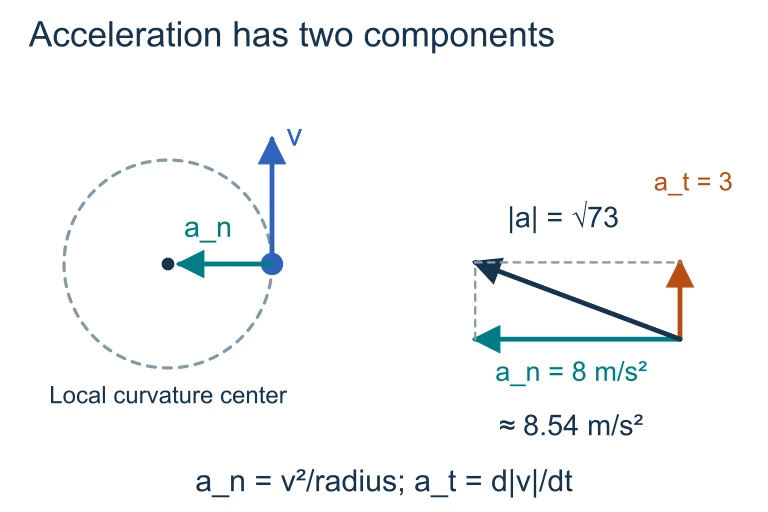 Velocity follows the local tangent to the path. Normal acceleration points toward the center of curvature, while tangential acceleration changes the speed.
SECTION 6
Worked Example — Projectile Launched from a Cliff
A ball is launched from the edge of a 45.0-m-high cliff with an initial speed of 30.0 m/s at an angle of 37.0° above the horizontal. We wish to find (a) the time of flight until the ball hits the ground below the cliff, (b) the horizontal range, and (c) the speed at impact. Take g = 9.80 m/s².
Projectile from an Elevated Launch Point
- 1
Step 1 — Resolve Initial Velocity
Using the launch angle θ = 37.0°: v₀ₓ = v₀ cos θ = 30.0 × cos 37.0° = 30.0 × 0.7986 ≈ 23.96 m/s, and v₀ᵧ = v₀ sin θ = 30.0 × sin 37.0° = 30.0 × 0.6018 ≈ 18.05 m/s. The horizontal component remains constant throughout the flight.v₀ₓ ≈ 23.96 m/s, v₀ᵧ ≈ 18.05 m/s - 2
Step 2 — Establish Coordinate System
Place the origin at the launch point with +x horizontal (in the direction of launch) and +y upward. The initial position is (0, 0), and the ground is at y = −45.0 m. The vertical equation of motion becomes: y(t) = v₀ᵧ t − ½gt² = 18.05t − 4.90t².y = −45.0 m at impact - 3
Step 3 — Solve for Time of Flight
Set y(t) = −45.0: −45.0 = 18.05t − 4.90t². Rearranging: 4.90t² − 18.05t − 45.0 = 0. Apply the quadratic formula: t = [18.05 ± √(18.05² + 4 × 4.90 × 45.0)] / (2 × 4.90). The discriminant is 325.8 + 882.0 = 1207.8, so √1207.8 ≈ 34.75. Taking the positive root: t = (18.05 + 34.75) / 9.80 ≈ 52.80 / 9.80 ≈ 5.39 s.t ≈ 5.39 s - 4
Step 4 — Compute Horizontal Range
Since horizontal motion is uniform: x = v₀ₓ × t = 23.96 × 5.39 ≈ 129.1 m.R ≈ 129 m - 5
Step 5 — Find Speed at Impact
The horizontal velocity at impact is still vₓ = 23.96 m/s. The vertical velocity at impact: vᵧ = v₀ᵧ − gt = 18.05 − 9.80 × 5.39 = 18.05 − 52.82 ≈ −34.77 m/s (negative = downward). The speed is |v⃗| = √(vₓ² + vᵧ²) = √(23.96² + 34.77²) = √(574.1 + 1209.0) = √1783.1 ≈ 42.2 m/s. Alternatively, energy conservation gives the same result: ½mv² = ½mv₀² + mgh → v = √(v₀² + 2gh) = √(900 + 882) ≈ 42.2 m/s.v_impact ≈ 42.2 m/s
SECTION 7
Coordinate Systems & Representations Compared
A powerful aspect of multidimensional kinematics is the freedom to choose the coordinate system that best matches the geometry of the problem. Different representations can simplify the mathematics dramatically. The table below compares three common coordinate frameworks encountered in AP Physics C: Mechanics.
| Coordinate System | Best For | Position Vector | Key Advantage |
|---|---|---|---|
| Cartesian (x, y, z) | Projectile motion, linear acceleration problems | r⃗ = x î + y ĵ + z k̂ | Components decouple when acceleration is along an axis |
| Polar (r, θ) | Circular motion, central-force orbits | r⃗ = r r̂ | Natural for radially symmetric problems; centripetal term arises automatically |
| Tangential-Normal (s, n) | General curvilinear paths, road design | Path parameterized by arc length s | Separates speed changes (tangential) from direction changes (normal) cleanly |
Comparison of coordinate systems for multidimensional kinematics
KEY TAKEAWAY
SECTION 8
Connections to Advanced Dynamics
Everything we have developed so far assumes either constant acceleration (projectile motion) or a specific constraint like circular motion. In reality, forces—and therefore accelerations—often vary with position, velocity, or time. The machinery of vector kinematics extends seamlessly to these cases, but closed-form solutions are no longer guaranteed and numerical integration or more advanced analytical methods become necessary. The table below contrasts the constant-acceleration regime with the general case.
| Feature | Constant Acceleration (AP C Focus) | Variable Acceleration (Advanced) |
|---|---|---|
| Equation of motion | r⃗(t) = r⃗₀ + v⃗₀t + ½a⃗t² | r⃗(t) = r⃗₀ + ∫v⃗ dt, solved via differential equations or numerical methods |
| Trajectory shape | Parabola (projectile), circle (uniform circular) | Ellipses (Kepler orbits), spirals, chaotic paths |
| Solving technique | Algebraic (quadratic formula, trigonometry) | Separation of variables, Lagrangian mechanics, Runge-Kutta integration |
| AP C exam relevance | Directly tested in MCQ and FRQ | Occasionally tested when a(t) or a(v) is given and you must integrate |
Constant vs. variable acceleration in multidimensional kinematics
On the AP Physics C exam, you may encounter problems where acceleration is a given function of time, such as a⃗(t) = (αt) î + (β) ĵ. In these cases, the strategy is to integrate a⃗(t) with respect to time to obtain v⃗(t), applying the initial condition v⃗(0) = v⃗₀, and then integrate again to obtain r⃗(t). This direct application of the fundamental theorem of calculus is the bridge between the constant-acceleration toolkit and the more general framework of Newtonian dynamics that dominates the remainder of the AP C: Mechanics curriculum.
Exam Strategy
SECTION 9
Practice Problems
Question 1: CONCEPTUAL
- A. Both velocity and acceleration are zero.
- B. Velocity is horizontal and nonzero; acceleration is zero.
- C. Velocity is horizontal and nonzero; acceleration is g downward.
- D. Velocity is zero; acceleration is g downward.
Show answer (C)
Question 2: BASIC CALCULATION
- A. 2 m/s²
- B. 2√10 m/s²
- C. 6 m/s²
- D. 10 m/s²
Show answer (B)
Question 3: INTERMEDIATE
- A. 3.00 m/s²
- B. 8.00 m/s²
- C. 8.54 m/s²
- D. 11.0 m/s²
Show answer (C)
Question 4: APPLIED
10 ptsShow answer
Question 5: CRITICAL THINKING
7 ptsShow answer
SUMMARY
Key Concepts in Motion in Two or Three Dimensions
Summary
Motion in multiple dimensions is described by treating the position vector r⃗(t) as a vector-valued function of time. The velocity v⃗ = dr⃗/dt is tangent to the trajectory, and the acceleration a⃗ = dv⃗/dt governs how both speed and direction change. The independence of components in Cartesian coordinates allows each dimension to be solved separately and then recombined. For projectile motion (constant a⃗ = −g ĵ), this yields parabolic trajectories described by r⃗(t) = r⃗₀ + v⃗₀t + ½a⃗t².
For circular and curvilinear motion, the acceleration decomposes into a tangential component at = dv/dt (changing speed) and a centripetal component ac = v²/r (changing direction). When acceleration varies with time, integration of a⃗(t) with appropriate initial conditions yields velocity and position. Choosing the right coordinate system—Cartesian, polar, or tangential-normal—can dramatically simplify the mathematical analysis.