Connecting Linear and Rotational Motion - AP Physics C Mechanics

SECTION 1

Historical Context & Motivation

The connection between linear (translational) motion and rotational motion is one of the most elegant structural parallels in classical mechanics. For centuries, physicists studied falling bodies and spinning wheels as if they inhabited separate theoretical worlds. The realization that a single set of mathematical relationships—linking arc length to angle, tangential speed to angular velocity, and tangential acceleration to angular acceleration—could bridge those two domains transformed mechanics from a collection of special cases into a unified discipline. Understanding this bridge is essential not only for solving rigid-body problems on the AP Physics C exam but also for grasping how real machines, from car transmissions to gyroscopes, actually work.

1687 • Newton's Principia

Isaac Newton published the Principia Mathematica, establishing the laws of linear motion (F = ma) and laying the groundwork for extending force concepts to rotation via torque.

1736 • Euler's Rigid-Body Mechanics

Leonhard Euler formalized the equations of rotational dynamics, introducing the moment of inertia and the rotational analog τ = Iα, explicitly mirroring Newton's second law.

1834 • Hamilton & Lagrange Unification

Lagrangian mechanics treated translational and rotational coordinates on equal footing using generalized coordinates, revealing that the linear–rotational analogy is not merely pedagogical but structurally deep.

1900s • Engineering Applications

The rolling-without-slipping constraint became central to automotive, aerospace, and robotics engineering, making the linear–rotational connection an indispensable practical tool.

The central question this lesson addresses is straightforward but profound: How do we translate between the language of displacement, velocity, and acceleration (linear) and the language of angle, angular velocity, and angular acceleration (rotational)? Mastering this translation will let you attack any problem involving wheels, pulleys, gears, or rolling objects with confidence.

SECTION 2

Core Principles & Definitions

At the heart of this topic lies a set of direct analogies between translational and rotational quantities, connected by the radius of the circular path. Each translational variable has a rotational counterpart, and a simple multiplicative factor of r (the distance from the axis of rotation) links the two. These relationships are not merely convenient shortcuts—they follow directly from the definition of the radian as a ratio of arc length to radius. The four foundational ideas below form the conceptual skeleton of the entire lesson.

Arc Length – Angle Relation

The arc length s traversed by a point on a rotating body equals rθ, where θ is measured in radians. This is the geometric foundation of all linear–rotational connections.

Tangential Velocity

Differentiating s = rθ with respect to time gives v_t = rω. The tangential speed of any point on a rigid body is proportional to its radial distance from the axis.

Tangential Acceleration

A second differentiation yields a_t = rα. This tangential component changes the speed of the point, while the centripetal component a_c = ω²r changes its direction.

Rolling Without Slipping

When a body rolls without slipping, the contact point has zero velocity relative to the surface. This constraint locks together the translational velocity of the center of mass and the angular velocity: v_cm = Rω.

✦

KEY TAKEAWAY

Think of a record player. Every point on the vinyl shares the same angular velocity ω, but a point near the rim travels a much longer arc per revolution than one near the center. That difference in linear speed is entirely captured by a single factor: the radius r. The relationships s = rθ, v_t = rω, and a_t = rα are just three faces of that same geometric fact. Master the radius as the 'exchange rate' between linear and angular quantities, and the rest follows naturally.

SECTION 3

Visual Explanation

The diagram below illustrates a rigid disk rotating about a fixed axis through its center. Two points—one at radial distance r₁ and one at r₂—are highlighted to show how the same angular velocity produces different tangential velocities. Notice that the tangential velocity vectors are always perpendicular to the radii and scale linearly with distance from the center.

The dashed circles represent the paths of two points at radii r₁ (violet) and r₂ (pink). The upward arrows show tangential velocity vectors whose magnitudes are proportional to the respective radii. Both points share the same angular velocity ω.

This diagram captures the essential geometry: the tangential velocity vector at each point is perpendicular to the radius and has magnitude v = rω. Because both points are part of the same rigid body, they rotate through the same angle in the same time, meaning they share identical ω. The outer point simply covers more linear distance per revolution. This insight generalizes: any kinematic quantity with dimensions of length (arc length, tangential speed, tangential acceleration) is obtained by multiplying the corresponding angular quantity by the radial distance r.

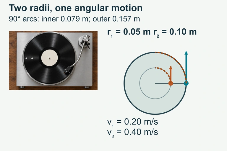At the illustrated instant, ω = 4 rad/s. Points at radii 0.05 m and 0.10 m move at 0.20 m/s and 0.40 m/s. A shared 90° rotation traces arcs of 0.0785 m and 0.1571 m. The required companion adds the instantaneous tangential accelerations.

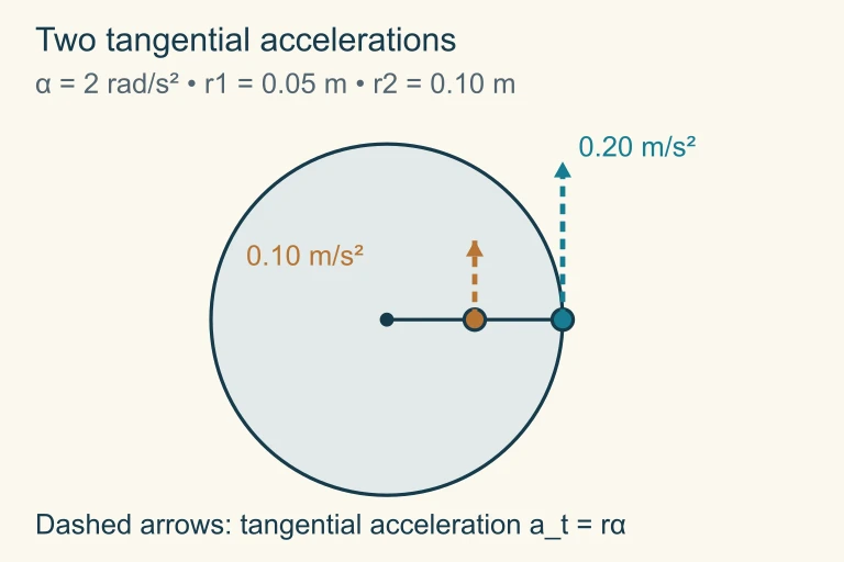At the instant shown, ω = 4 rad/s and α = 2 rad/s². Both points share angular motion; v = rω and a_t = rα, so the outer point has twice the speed and twice the tangential acceleration. The 90° arc lengths are 0.0785 m and 0.1571 m.

A launched metal cylinder on a track with a prominent colored band and a magnified rubbing contact region. Kinetic friction slows the center of mass and increases the spin of an initially nonspinning solid cylinder. Slipping ends when v = Rω; one-third of the initial mechanical energy has been dissipated in this model.

Kinetic friction brings translation and spin together. Kinetic friction slows the center of mass and increases the spin of an initially nonspinning solid cylinder. Slipping ends when v = Rω; one-third of the initial mechanical energy has been dissipated in this model. Kinetic friction slows the center of mass and increases the spin of an initially nonspinning solid cylinder. Slipping ends when v = Rω; one-third of the initial mechanical energy has been dissipated in this model.

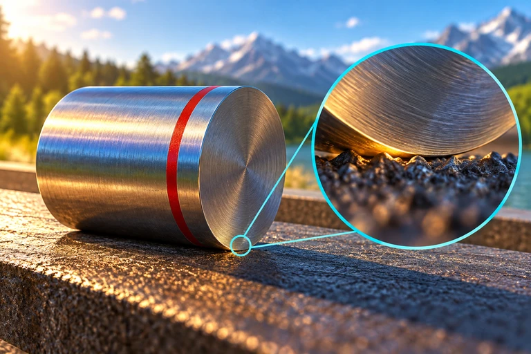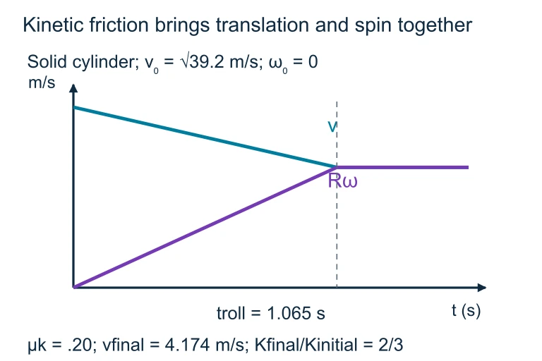Spin-up states have computed positions and rotations. Kinetic friction slows the center of mass and increases the spin of an initially nonspinning solid cylinder. Slipping ends when v = Rω; one-third of the initial mechanical energy has been dissipated in this model. 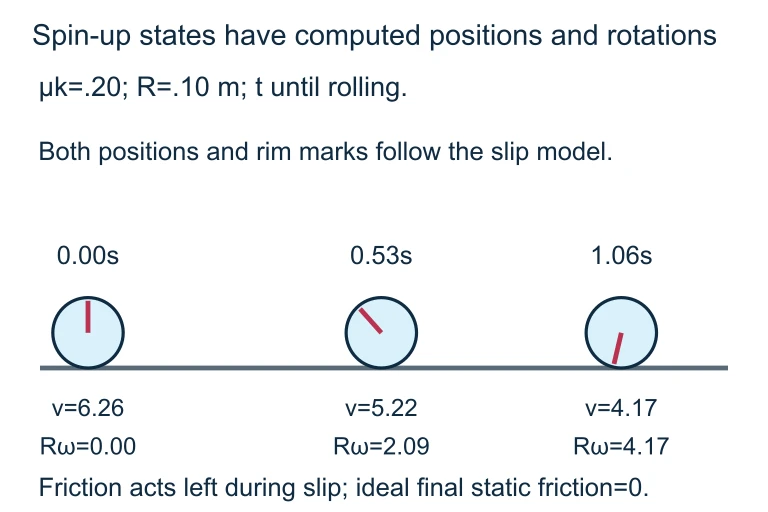Kinetic friction slows the center of mass and increases the spin of an initially nonspinning solid cylinder. Slipping ends when v = Rω; one-third of the initial mechanical energy has been dissipated in this model.

SECTION 4

Mathematical Framework

Let us now derive the three fundamental bridge equations and the rolling constraint rigorously. All derivations start from a single geometric definition—the radian—and proceed by successive differentiation with respect to time. We assume the axis of rotation is fixed and that r is constant for a given point on a rigid body.

ARC LENGTH – ANGLE

s = rθ

Where s is the arc length (m), r is the radial distance from the rotation axis (m), and θ is the angular displacement (rad). This equation is valid only when θ is in radians—a key exam pitfall.

TANGENTIAL VELOCITY

v_t = ds/dt = r(dθ/dt) = rω

Taking the time derivative of s = rθ (with r constant for a fixed point on a rigid body) yields the tangential velocity. Here ω = dθ/dt is the angular velocity in rad/s.

TANGENTIAL ACCELERATION

a_t = dv_t/dt = r(dω/dt) = rα

Differentiating once more gives the tangential (linear) acceleration, where α = dω/dt is the angular acceleration in rad/s². This component is tangent to the circular path and changes the speed of the point.

CENTRIPETAL ACCELERATION

a_c = v_t²/r = ω²r

The centripetal (radial) acceleration points toward the center and changes the direction of velocity without changing its magnitude. The total linear acceleration of the point is the vector sum: a = √( $a_t$ ² + $a_c$ ²).

The Rolling-Without-Slipping Constraint

When a wheel or sphere rolls without slipping on a surface, the instantaneous velocity of the contact point relative to the surface is zero. This imposes a powerful kinematic constraint: v_cm = Rω, where v_cm is the translational speed of the center of mass and R is the radius of the rolling body. Differentiating yields a_cm = Rα. This constraint is essential for solving inclined-plane rolling problems, Atwood machines with massive pulleys, and any scenario where rotation and translation are coupled. On the AP exam, recognizing when to apply (or not apply) this constraint is often the decisive step in a free-response question.

SECTION 5

The Linear–Rotational Analogy in Full

One of the most powerful study strategies for AP Physics C is to internalize the complete correspondence table between translational and rotational quantities. Every kinematic equation, every dynamical law, and every energy expression has a rotational counterpart obtained by systematic substitution. The table below organizes these parallels and serves as a reference you should know cold by exam day.

Concept	Translational	Rotational	Bridge Equation
Displacement	s (m)	θ (rad)	s = rθ
Velocity	v (m/s)	ω (rad/s)	v = rω
Acceleration	a (m/s²)	α (rad/s²)	a = rα
Inertia	m (kg)	I (kg·m²)	I = Σmᵢrᵢ²
Force / Torque	F (N)	τ (N·m)	τ = rF sin θ
Newton's 2nd Law	F = ma	τ = Iα	—
Kinetic Energy	½mv²	½Iω²	—
Momentum	p = mv	L = Iω	—

Complete linear–rotational analogy table for AP Physics C

A sphere rolls without slipping down an incline. The center-of-mass velocity v_cm is locked to the angular velocity ω by the constraint v_cm = Rω. The contact point has zero velocity relative to the surface, and the total kinetic energy includes both translational and rotational terms.

The incline diagram above is the canonical AP Physics C setup. When a ball or cylinder rolls down a frictionless-looking ramp, students often forget that static friction is required to prevent slipping and to provide the torque that spins the object. However, static friction does no work (the contact point has zero velocity), so energy methods remain clean. The total kinetic energy is K = ½mv²_cm + ½Iω², and the rolling constraint lets you express everything in terms of a single variable.

SECTION 6

Worked Example: Solid Sphere Rolling Down an Incline

A solid sphere of mass m = 2.0 kg and radius R = 0.10 m starts from rest at the top of a ramp of height h = 3.0 m and rolls without slipping to the bottom. Find the translational speed of the center of mass and the angular velocity at the bottom.

Solid Sphere Rolling Down a Ramp

1
Step 1 — Identify known quantities and the approach

We have m = 2.0 kg, R = 0.10 m, h = 3.0 m, and v₀ = 0. Because static friction does no work during rolling without slipping, we can use conservation of mechanical energy: mgh = ½mv²_cm + ½Iω². The moment of inertia of a solid sphere about its center is I = (2/5)mR².
2
Step 2 — Apply the rolling constraint

Since the sphere rolls without slipping, v_cm = Rω, so ω = v_cm/R. Substituting into the energy equation: mgh = ½mv² + ½ × (2/5)mR² × (v/R)² = ½mv² + (1/5)mv² = (7/10)mv².
3
Step 3 — Solve for v_cm

Canceling m from both sides: gh = (7/10)v². Solving: v² = 10gh/7, so v = √(10gh/7) = √(10 × 9.8 × 3.0 / 7) = √(42.0) ≈ 6.48 m/s.

v_cm ≈ 6.5 m/s
4
Step 4 — Find angular velocity

Using the rolling constraint: ω = v_cm / R = 6.48 / 0.10 = 64.8 rad/s.

ω ≈ 65 rad/s
5
Step 5 — Verify and interpret

Note that v_cm ≈ 6.5 m/s is less than √(2gh) ≈ 7.67 m/s (the speed of a frictionless sliding block). The 'missing' kinetic energy has been channeled into rotational kinetic energy. Specifically, K_rot/K_total = (2/5)/(1 + 2/5) = 2/7 ≈ 28.6% of the total kinetic energy is rotational.

SECTION 7

Common Pitfalls & Exam Tips

Students frequently lose points on AP Physics C free-response questions not from a lack of understanding but from specific, predictable mistakes in applying the linear–rotational bridge. The table below catalogs the most common pitfalls alongside the correct approach.

Common Pitfall	Why It's Wrong	Correct Approach
Using degrees in s = rθ	The radian is defined as arc length / radius; the equation only holds in radians.	Always convert to radians first: θ(rad) = θ(°) × π/180.
Forgetting rotational KE	Rolling objects carry both ½mv² and ½Iω²; omitting the latter yields too-fast speeds.	Write K_total = ½mv² + ½Iω² and use the rolling constraint to combine.
Applying v = Rω when slipping occurs	The constraint v_cm = Rω only holds for rolling without slipping. With kinetic friction, v_cm ≠ Rω.	Check whether the problem states 'rolls without slipping.' If not, treat v_cm and ω as independent.
Confusing $a_t$ with $a_c$	Tangential acceleration changes speed ( $a_t$ = rα); centripetal acceleration changes direction ( $a_c$ = ω²r). Mixing them gives wrong net acceleration.	Draw a diagram. $a_t$ is tangent to the path; $a_c$ points radially inward. Compute \|a\| = √( $a_t$ ² + $a_c$ ²).
Using wrong moment of inertia	Solid sphere (2/5 mR²), hollow sphere (2/3 mR²), disk (1/2 mR²), and hoop (mR²) each give different results.	Memorize or derive the standard moments. The exam formula sheet provides some but not all.

Common exam pitfalls when connecting linear and rotational motion

⚡

EXAM STRATEGY

On free-response questions involving rolling, always start by (1) drawing a free-body diagram that includes friction at the contact point, (2) writing Newton's second law for translation (ΣF = ma_cm) and for rotation (Στ = Iα) separately, and (3) linking them with the rolling constraint a_cm = Rα. This systematic three-equation approach earns maximum partial credit even if you make an algebra error downstream.

SECTION 8

Connection to Advanced Theory

The linear–rotational bridge you have learned is a special case of far more general principles encountered in intermediate and advanced mechanics. Recognizing where these ideas lead helps contextualize the AP-level treatment and motivates deeper study. The table below compares the AP framework with the corresponding advanced formulations.

AP Physics C Treatment	Advanced / University Treatment
v = rω for a point on a rigid body rotating about a fixed axis	v = ω × r (vector cross product), generalizing to three-dimensional rotation about any axis
I = Σmᵢrᵢ² (scalar moment about a single axis)	The inertia tensor I is a 3×3 matrix; the scalar I is just one diagonal element for a principal axis
τ = Iα along a fixed axis	Euler's equations: τ = dL/dt in the body frame, accounting for precession and nutation
Energy: ½mv² + ½Iω² with rolling constraint	Lagrangian mechanics: L = T − V with generalized coordinates (θ, x_cm) and holonomic constraint x = Rθ

AP-level vs. advanced rotational dynamics

In the Lagrangian formulation, the rolling-without-slipping constraint appears as a holonomic constraint of the form x − Rθ = constant, which can be directly substituted into the Lagrangian to reduce the number of degrees of freedom. This is exactly what you do at the AP level when you replace ω with v/R—you are performing constraint substitution, a technique that scales seamlessly to much more complex systems. Understanding the AP treatment well thus provides genuine preparation for intermediate classical mechanics courses (e.g., Taylor or Morin), where the same logic is simply extended to more dimensions and more general constraints.

SECTION 9

Practice Problems

Question 1: CONCEPTUAL

A solid disk and a hollow ring of equal mass and radius are released from rest at the top of the same incline and roll without slipping. Which reaches the bottom first, and why?

A. The ring arrives first because its greater moment of inertia stores more energy in rotation, reducing friction losses.
B. They arrive at the same time because they have equal mass and start from the same height.
C. The disk arrives first because a smaller fraction of its gravitational potential energy goes into rotational kinetic energy, leaving more for translational speed.
D. The disk arrives first because its smaller moment of inertia means friction exerts a larger torque, spinning it faster down the ramp.

Show answer (C)

C is correct. For rolling without slipping, energy conservation gives mgh = ½mv² + ½Iω² = ½mv²(1 + I/(mR²)). The disk has I = ½mR², so the factor is 1 + ½ = 3/2, giving v = √(4gh/3). The ring has I = mR², so the factor is 1 + 1 = 2, giving v = √(gh). Since √(4gh/3) > √(gh), the disk is faster. A is wrong because a larger moment of inertia actually diverts more energy into rotation, slowing translation. B is wrong because equal mass and height do not guarantee equal translational speeds when rotational inertias differ. D is wrong because friction's role is to enforce the no-slip condition—not to accelerate the object; moreover, larger I actually means smaller angular acceleration for a given torque.

Question 2: BASIC CALCULATION

A wheel of radius 0.25 m rotates at a constant angular velocity of 12 rad/s. What is the tangential speed of a point on the rim, and what is the centripetal acceleration of that point?

A. v = 3.0 m/s, $a_c$ = 36 m/s²
B. v = 3.0 m/s, $a_c$ = 144 m/s²
C. v = 48 m/s, $a_c$ = 576 m/s²
D. v = 0.48 m/s, $a_c$ = 5.76 m/s²

Show answer (A)

A is correct. The tangential speed is v = rω = 0.25 × 12 = 3.0 m/s. The centripetal acceleration is

a_c

= ω²r = (12)² × 0.25 = 144 × 0.25 = 36 m/s². B incorrectly computes

a_c

= ω²r as (12)² × 1 = 144, effectively using r = 1 m instead of 0.25 m. C uses v = ω/r = 12/0.25 = 48, which inverts the relationship. D appears to compute v = rω with r and ω swapped as v = r²ω or similar—there is no standard formula that gives 0.48 m/s from these values.

Question 3: INTERMEDIATE

A string is wrapped around a uniform solid cylinder (mass M = 4.0 kg, radius R = 0.20 m) that is free to rotate about a fixed horizontal axis. A block of mass m = 1.5 kg hangs from the free end of the string. When the system is released from rest, find the linear acceleration of the block. (I_cylinder = ½MR²)

A. a = 4.2 m/s²
B. a = 9.8 m/s²
C. a = 2.7 m/s²
D. a = 5.6 m/s²

Show answer (A)

A is correct. For the block: mg − T = ma. For the cylinder: TR = Iα = ½MR²α. The string unwinds without slipping, so a = Rα, giving α = a/R. Substituting: T = ½MR²(a/R)/R = ½Ma. Now the block equation becomes mg − ½Ma = ma, so a = mg/(m + ½M) = (1.5 × 9.8)/(1.5 + 2.0) = 14.7/3.5 = 4.2 m/s². B ignores the rotational inertia of the cylinder entirely (as if the string just free-falls). C likely uses I = MR² (a hoop) instead of ½MR² for the cylinder, giving a = mg/(m + M) = 14.7/5.5 ≈ 2.7 m/s². D does not correspond to a standard error with these values and is included as a distractor.

Question 4: APPLIED

5 pts

A solid sphere of mass 0.50 kg and radius 0.060 m rolls without slipping along a horizontal surface at 4.0 m/s, then encounters a frictionless ramp. How far up the ramp (vertical height h) does the sphere travel before stopping? (I_sphere = 2/5 mR²)

Show answer

Point 1 (1 pt): Correctly identify that the total KE at the bottom includes both translational and rotational components: K = ½mv² + ½Iω². Point 2 (1 pt): Note that the ramp is frictionless, so the sphere cannot maintain rolling—angular velocity is conserved (no torque). The sphere slides up the ramp with its initial translational KE converting to potential energy, while the rotational KE remains constant as ½Iω². Point 3 (1 pt): Since only translational KE converts to PE: ½mv² = mgh, giving h = v²/(2g) = (4.0)²/(2 × 9.8) = 0.816 m. Point 4 (1 pt): Report h ≈ 0.82 m with correct units. Point 5 (1 pt): This is a common trick question. Many students incorrectly use mgh = ½mv² + ½Iω² = 7/10 mv², yielding h = 7v²/(10g) ≈ 1.14 m. This would only be correct if the ramp had sufficient friction to maintain rolling. Because the ramp is frictionless, no torque acts to decelerate the spin—the rotational KE never converts to PE. The correct answer is h ≈ 0.82 m.

Question 5: CRITICAL THINKING

7 pts

A uniform thin rod of mass M and length L is pivoted at one end and released from rest in a horizontal position. The moment of inertia of the rod about the pivot end is I = (1/3)ML². Let θ be the angle the rod makes with the horizontal as it swings downward, and let g be the acceleration due to gravity. (a) Derive an expression for the angular acceleration α of the rod as a function of the angle θ that the rod makes with the horizontal. Express your answer in terms of M, L, g, and θ. (b) Determine the tangential acceleration of the free end of the rod at the instant of release (θ = 0). Express your answer in terms of g. (c) Compare the tangential acceleration found in part (b) to the acceleration due to gravity g. Explain physically why the tip of the rod can accelerate faster than a freely falling object.

Show answer

Part (a) — Angular acceleration as a function of θ: Point 1 (1 pt): Correctly identify the torque about the pivot. Gravity acts at the center of mass (L/2 from the pivot). When the rod makes angle θ with the horizontal, the perpendicular component of the gravitational force provides a lever arm of (L/2)cos θ. So τ = Mg(L/2)cos θ. Point 2 (1 pt): Apply Newton's second law for rotation: τ = Iα. With I = (1/3)ML²: Mg(L/2)cos θ = (1/3)ML² α. Point 3 (1 pt): Solve for α: α = (3g cos θ)/(2L). Part (b) — Tangential acceleration of the free end at θ = 0: Point 4 (1 pt): At θ = 0, cos 0 = 1, so α = 3g/(2L). The free end is at distance r = L from the pivot. Point 5 (1 pt): The tangential acceleration of the free end is

a_t

= Lα = L × 3g/(2L) = 3g/2 = 1.5g ≈ 14.7 m/s². Part (c) — Comparison and physical significance: Point 6 (1 pt): The tangential acceleration of the tip (3g/2) exceeds the free-fall acceleration g. This means the tip of the rod accelerates downward faster than a freely falling object at the instant of release. Point 7 (1 pt): Physical explanation: The pivot exerts an upward reaction force on the rod near the hinge. By Newton's third law, the portion of the rod near the pivot is partially supported, so its gravitational acceleration is effectively reduced. The rotational constraint forces the entire rod to share a common angular acceleration, which means points farther from the pivot move faster (v = rω). The tip at distance L receives a disproportionately large share of the kinetic energy and thus accelerates faster than g. This is the same principle that allows a hinged meter stick to fall away from a ball balanced on its free end — the stick's tip outraces the freely falling ball.

SUMMARY

Lesson Summary

Summary

This lesson established the fundamental bridge between translational (linear) motion and rotational motion. The three core relationships—s = rθ, v = rω, and $a_t$ = rα—all flow from a single geometric fact: the radian measure relates arc length to radius. The centripetal acceleration $a_c$ = ω²r completes the picture by accounting for the change in direction of the velocity vector. For objects that roll without slipping, the constraint v_cm = Rω (and its derivative a_cm = Rα) locks the translational and rotational degrees of freedom together, enabling powerful energy-conservation and force-torque analyses.

On the AP Physics C exam, always begin rolling-body problems by writing Newton's second law for translation (ΣF = ma_cm) and Newton's second law for rotation (Στ = Iα) as two separate equations, then link them with the rolling constraint. Remember that static friction does no work during pure rolling, so energy methods remain valid. Watch for trick scenarios (like a frictionless ramp) where the constraint breaks. Mastery of these connections will prepare you for the majority of torque and rotational dynamics problems on the exam.