

SECTION 1
Historical Context & Motivation
Long before physicists formulated the modern concept of momentum, natural philosophers wrestled with a fundamental question: what quantity best characterizes a body in motion? The ancient notion of impetus—a kind of internal motive force imparted to a projectile—dominated medieval thinking. It was not until the Scientific Revolution that rigorous, quantitative treatments replaced these intuitive but imprecise ideas. The concept of impulse, the product of force and the time interval over which it acts, arose naturally once Newton cast his second law in its most general form—a form that deals not with acceleration alone, but with the rate of change of momentum.
1644 • Descartes' Quantity of Motion
1687 • Newton's Principia
1743 • d'Alembert's Principle
1900s • Modern Applications
The central question this lesson addresses is deceptively simple: if we know the net force on an object as a function of time, how do we calculate the resulting change in its momentum? And conversely, if we observe a momentum change, what can we infer about the force that produced it? These two perspectives—force-to-motion and motion-to-force—form the heart of the impulse–momentum theorem, and mastering them is essential for every AP Physics C student.
SECTION 2
Core Principles & Definitions
Before diving into the mathematics, it is crucial to establish a precise vocabulary. In everyday language "momentum" and "impulse" are used loosely, but in physics each term carries a sharply defined meaning rooted in Newton's second law. The following foundational ideas form the scaffolding for everything that follows.
Linear Momentum (p⃗)
Net Force as dp⃗/dt
Impulse (J⃗)
Impulse–Momentum Theorem
Average Force
KEY TAKEAWAY
SECTION 3
Force–Time Diagrams & Impulse as Area
One of the most powerful representations in momentum analysis is the force versus time graph. Because impulse is defined as the integral J = ∫F dt, the impulse delivered to an object is geometrically equal to the area under the F(t) curve. This graphical interpretation is indispensable on the AP exam, where force–time data are frequently given in graph form and you must extract the impulse by computing that area.
In the diagram above, the force profile is trapezoidal: a linear ramp from 0 to 2000 N over 2 ms, a 2 ms plateau at 2000 N, and a linear ramp back to 0 over another 2 ms. The total area consists of two triangles (each with area ½ × 2 × 10⁻³ s × 2000 N = 2.0 N·s) and one rectangle (2 × 10⁻³ s × 2000 N = 4.0 N·s), giving J = 2.0 + 4.0 + 2.0 = 8.0 N·s. This graphical approach—decomposing the area into simple geometric shapes—is the method you will use most often on the AP exam when the force is given as a piecewise-linear function of time. When the force is given as an analytic function, you will instead evaluate the integral directly.
SECTION 4
Mathematical Framework
The impulse–momentum theorem follows directly from Newton's second law through a straightforward integration. Starting from the vector form of the second law and integrating both sides over the time interval of interest, we arrive at an exact relationship between the net impulse and the resulting momentum change. Let us develop this derivation carefully, because variations of it appear routinely on the AP Physics C exam.
NEWTON'S SECOND LAW (GENERAL FORM)
F⃗_net is the net external force, p⃗ is the linear momentum, m is the mass, and v⃗ is the velocity. When m is constant, this reduces to F⃗_net = ma⃗.
IMPULSE DEFINITION (INTEGRAL FORM)
J⃗ is the net impulse vector. The integral is taken over the full interaction time from to . Units: N·s = kg·m/s.
IMPULSE–MOMENTUM THEOREM
Derived by integrating both sides of F⃗_net = dp⃗/dt: ∫F⃗ dt = ∫dp⃗ = p⃗_f − p⃗_i. This is an exact vector equation valid for any time-varying force, assuming constant mass.
AVERAGE FORCE
When you cannot resolve F(t) in detail, the average force provides the constant-force equivalent. This is especially useful in collision analysis where the force profile is unknown but the duration and velocity change are measurable.
It is worth emphasizing that the impulse–momentum theorem is not a separate postulate; it is a mathematical consequence of Newton's second law. Any problem solvable via F = ma can, in principle, be recast as an impulse problem, but the impulse formulation is particularly advantageous in two scenarios: (1) when the force varies with time in a way that makes direct acceleration analysis cumbersome, and (2) when the interaction time is very short (collisions), so that the net impulse captures the entire effect of a complicated force profile in a single integral.
AP Exam Tip
SECTION 5
Impulse in Collisions — Extending Contact Time
One of the most practically significant consequences of the impulse–momentum theorem is its implication for collision safety. When an object undergoes a given change in momentum Δp, the impulse J = Δp is fixed regardless of how the collision unfolds. Since J = F_avg × Δt, increasing the contact time Δt necessarily decreases the average force experienced by the object. This principle underlies automotive crumple zones, airbags, helmet padding, and even the technique of "giving" with a catch in baseball—all of which work by extending the collision duration to reduce peak forces.
The side-by-side comparison above illustrates this vividly. Both triangular force profiles enclose the same area—24 N·s—so the momentum change is identical. However, the hard collision concentrates that impulse into 4 ms, generating a peak force three times larger than the soft collision, which spreads the same impulse over 12 ms. This is precisely why the AP exam might ask you to explain how a design modification (e.g., adding padding) reduces injury risk: the change in momentum is dictated by the initial and final velocities alone, so the only way to reduce F_avg is to increase Δt.
DESIGN PRINCIPLE
SECTION 6
Worked Example — Variable Force Impulse
Let us work through a problem that requires integration of a time-dependent force, a standard AP Physics C skill. This example illustrates the full mathematical procedure from force function to final velocity.
A 2.0 kg block, initially at rest on a frictionless surface, is struck by a force F(t) = (600 N/s)t − (100 N/s²)t² for 0 ≤ t ≤ 4.0 s. Find (a) the impulse delivered, (b) the final velocity, and (c) the average force during the interaction.
- 1
Step 1 — Identify Given Values
Mass m = 2.0 kg, initial velocity = 0 m/s, force function F(t) = 600t − 100t² (in SI units), and the time interval is t = 0 to t = 4.0 s. The motion is one-dimensional, so we work with scalar equations along the direction of F. - 2
Step 2 — Compute the Impulse via Integration
J = ∫₀⁴ (600t − 100t²) dt = [300t² − (100/3)t³] evaluated from 0 to 4. Substituting: J = 300(16) − (100/3)(64) = 4800 − 6400/3 = 4800 − 2133.3 = 2666.7 N·s.J ≈ 2667 N·s - 3
Step 3 — Apply the Impulse–Momentum Theorem
By the impulse–momentum theorem, J = Δp = mv_f − mv_i. Since = 0: = J / m = 2666.7 / 2.0 = 1333.3 m/s.≈ 1333 m/s - 4
Step 4 — Calculate the Average Force
F_avg = J / Δt = 2666.7 N·s / 4.0 s = 666.7 N. This is the constant force that, if applied for 4.0 s, would produce the same impulse and therefore the same momentum change.F_avg ≈ 667 N - 5
Step 5 — Reasonableness Check
The force function F(t) = 600t − 100t² equals zero at t = 0 and t = 6 s, reaching a maximum of F(3) = 900 N at t = 3 s. Our average of 667 N is below the peak but above zero, which is consistent. The impulse is positive, yielding a positive final velocity in the direction of the applied force—also consistent.
Common Mistake
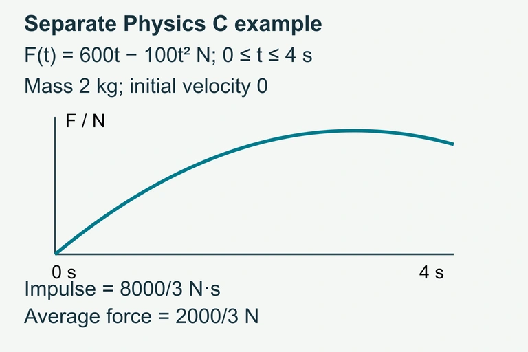 Separate idealized Physics C example: impulse is the force–time integral. With mass 2 kg starting from rest, the model implies a final speed of 4000/3 m/s.
SECTION 7
Impulse vs. Work — Two Sides of Force
Students often conflate impulse and work because both involve force. However, they capture fundamentally different aspects of a force's effect. Impulse (J = ∫F dt) measures how much a force changes an object's momentum, whereas work (W = ∫F·dx) measures how much a force changes an object's kinetic energy. The following table clarifies the distinction.
| Feature | Impulse (J⃗) | Work (W) |
|---|---|---|
| Definition | ∫F⃗ dt | ∫F⃗ · dr⃗ |
| Scalar or Vector? | Vector | Scalar |
| Quantity changed | Momentum (p⃗) | Kinetic energy (K) |
| Relevant theorem | Impulse–Momentum | Work–Energy |
| Integration variable | Time (dt) | Displacement (dr⃗) |
| Units | N·s = kg·m/s | N·m = J (joules) |
| Best used when... | Time interval or velocity change is known | Displacement or speed change is known |
Impulse vs. Work: contrasting two fundamental effects of force
STRATEGIC CHOICE ON THE EXAM
SECTION 8
Connections to Conservation Laws & Beyond
The impulse–momentum theorem is the single-object version of a far more powerful statement: the conservation of linear momentum for a system. When the net external force on a system is zero, the total impulse on the system is zero, and therefore total momentum is conserved. This link between impulse and conservation is the conceptual backbone of collision analysis, which occupies a significant portion of the AP Physics C curriculum.
| Concept | Impulse–Momentum (This Lesson) | Conservation of Momentum (Advanced) |
|---|---|---|
| Applies to | A single object under a known net force | A system of objects with zero net external force |
| Key equation | J⃗ = Δp⃗ = mv⃗_f − mv⃗_i | p⃗_system,i = p⃗_system,f |
| When to use | External force is known (or its time integral) | Internal forces dominate; external forces negligible |
| Derivation root | Newton's 2nd Law: F⃗ = dp⃗/dt | Newton's 3rd Law + 2nd Law for each body |
| Variable-mass extension | Rocket equation (thrust = × dm/dt) | Still holds for the rocket + exhaust system |
From impulse–momentum to conservation of momentum
Looking beyond the AP C curriculum, the impulse concept generalizes elegantly into Lagrangian and Hamiltonian mechanics, where the generalized impulse (∫ dt) drives changes in generalized momenta. In relativistic mechanics, the four-vector formulation of impulse accounts for the velocity-dependent mass (Lorentz factor γ), but the core theorem J = Δp retains its structure. Even in quantum field theory, the transfer of four-momentum between particles in scattering events is essentially an impulse concept—testifying to the extraordinary durability of the ideas you are learning in this lesson.
SECTION 9
Practice Problems
Question 1: CONCEPTUAL
- A. The ball that sticks, because it transfers all of its kinetic energy to the wall
- B. The ball that bounces, because its momentum reverses direction, yielding |Δp| = 2mv
- C. Both experience the same impulse, because they have the same mass and initial speed
- D. It depends on the elasticity of the wall, which is not specified
Show answer (B)
Question 2: BASIC CALCULATION
- A. 6 650 N
- B. 7 960 N
- C. 11 500 N
- D. 13 800 N
Show answer (C)
Question 3: INTERMEDIATE
- A. 8.0 m/s
- B. 10.0 m/s
- C. 12.0 m/s
- D. 16.0 m/s
Show answer (C)
Question 4: APPLIED
4 ptsShow answer
Question 5: CRITICAL THINKING
4 ptsShow answer
SUMMARY
Summary — Change in Momentum and Impulse
Summary
The impulse–momentum theorem states that the net impulse on an object equals its change in momentum: J⃗ = Δp⃗ = mv⃗_f − mv⃗_i. Impulse is computed as the time integral of force, J⃗ = ∫F⃗ dt, which corresponds geometrically to the area under a force–time curve. When the exact F(t) is unknown, the average force is defined as F_avg = Δp/Δt.
For a fixed momentum change, extending the contact time reduces the peak and average forces—the principle behind airbags, crumple zones, and protective padding. Unlike work (which changes kinetic energy via ∫F·dx), impulse changes momentum via ∫F dt. On the AP exam, choose the impulse approach whenever time-domain information is provided, and always establish a clear sign convention before computing Δp.