The Doppler Effect - AP Physics 2

SECTION 1

Historical Context & Motivation

Anyone who has stood near a roadway and heard the pitch of a siren change as an ambulance approaches and then recedes has experienced one of the most intuitive wave phenomena in physics. The observation that relative motion between a wave source and an observer alters the detected frequency was first placed on a firm theoretical footing in the nineteenth century, but its implications now span disciplines from astrophysics to medical imaging. Understanding the historical arc of this discovery reveals how a single physical insight can generate an extraordinary range of technologies.

1842 • Doppler's Hypothesis

Austrian physicist Christian Doppler published a paper proposing that the observed frequency of a wave depends on the relative velocity of source and observer. He initially applied his idea to starlight, suggesting that the color of stars was influenced by their motion.

1845 • Buys Ballot's Confirmation

Dutch meteorologist Christophorus Buys Ballot tested Doppler's prediction using a group of horn players on a moving train near Utrecht. Listeners at the station confirmed a noticeable pitch shift, providing the first experimental verification of the acoustic Doppler effect.

1868 • Huggins & Stellar Spectroscopy

William Huggins measured the Doppler shift in spectral lines of the star Sirius, establishing the first radial velocity measurement of a star and extending the effect to electromagnetic waves.

1929 • Hubble's Expanding Universe

Edwin Hubble used redshift data—frequency shifts of light from distant galaxies—to demonstrate that the universe is expanding. The Doppler effect became a cornerstone of modern cosmology.

1960s • Medical & Radar Applications

Doppler ultrasound entered clinical medicine, enabling non-invasive measurement of blood flow velocities. Simultaneously, police radar guns and weather Doppler radar became standard tools, demonstrating the practical breadth of the phenomenon.

The central question that Doppler's work addressed is deceptively simple: when a wave source and an observer are not stationary relative to one another, what frequency does the observer actually detect? Answering this question requires careful reasoning about how wavefronts accumulate in space, and the resulting equations connect directly to applications on the AP Physics 2 exam.

SECTION 2

Core Principles & Definitions

The Doppler effect arises from a fundamental property of wave propagation: once a wavefront is emitted, it travels through the medium at a speed determined by the medium's properties, regardless of any subsequent motion of the source. When a source moves toward an observer, each successive wavefront is emitted from a position slightly closer to the observer, compressing the wavelength and raising the perceived frequency. Conversely, when the source moves away, wavefronts are stretched apart, producing a lower detected frequency. The same logic applies when the observer moves relative to a stationary source, though the mathematical form differs slightly because the observer's motion changes the rate at which wavefronts are encountered.

Source Frequency (f₀)

The frequency at which the source actually vibrates and emits wavefronts, sometimes called the emitted frequency. This value is fixed by the source and is independent of the observer's motion.

Observed Frequency (f)

The frequency the observer detects, which may be higher or lower than f₀ depending on the relative motion between source and observer.

Wave Speed (v)

The speed at which wavefronts propagate through the medium. For sound in air at 20 °C, v ≈ 343 m/s. This speed depends on the medium, not on the source or observer velocity.

Approach → Higher Frequency

When the distance between source and observer is decreasing, the observed wavelength is compressed, and the observer perceives a higher frequency (blueshift).

Recession → Lower Frequency

When the distance is increasing, wavefronts are stretched, and the observer perceives a lower frequency (redshift).

✦

KEY TAKEAWAY

Think of wavefronts like letters mailed from a moving train. If the train travels toward your mailbox, each letter is mailed from a closer location, so letters arrive more frequently—even though the sender mails them at the same rate. If the train moves away, letters arrive less often. The actual mailing rate never changes; only the arrival rate at the observer does. This is the essence of the Doppler effect: relative motion compresses or stretches the spacing between successive wavefronts without altering the wave's propagation speed.

SECTION 3

Visual Explanation

In this diagram the pink dot represents a sound source moving to the right. The cyan circles show compressed wavefronts ahead of the source, leading Observer A to detect a higher frequency. The amber circles show stretched wavefronts behind the source, so Observer B detects a lower frequency.

The diagram above captures the essential geometry of the Doppler effect for a source moving through a medium. Notice that every wavefront travels outward at the same speed v, but because the source has shifted position between emissions, the centers of the circular wavefronts are not concentric. Ahead of the source the wavefronts bunch together, reducing the effective wavelength λ and raising the frequency f = v/λ that Observer A detects. Behind the source the wavefronts spread out, increasing λ and lowering the frequency heard by Observer B. The source's own vibration rate, f₀, has not changed—only the spatial distribution of wavefronts in the medium has been altered by the source's motion.

SECTION 4

Mathematical Framework

The AP Physics 2 exam focuses on the general Doppler equation for sound waves, which accounts for the motion of both the source and the observer through the medium. Deriving this expression begins with the recognition that the wave speed in the medium is fixed: once a wavefront leaves the source, it propagates at speed v regardless of what the source does next. We consider the one-dimensional case in which source and observer lie along a single line.

GENERAL DOPPLER EQUATION (SOUND)

f = f₀ × (v ± v_o) / (v ∓ v_s)

f = observed frequency, f₀ = source frequency, v = speed of sound in the medium, v_o = observer speed, v_s = source speed. Upper signs apply when source and observer approach each other; lower signs apply when they move apart.

💡

Sign Convention Tip

Rather than memorizing ± and ∓, use a physical reasoning approach. To increase the observed frequency the fraction must become larger, which means making the numerator larger (observer moving toward source: add v_o) and the denominator smaller (source moving toward observer: subtract v_s). Reverse the logic for a decrease.

Special Cases

MOVING SOURCE, STATIONARY OBSERVER

f = f₀ × v / (v ∓ v_s)

Observer is at rest (v_o = 0). Subtract v_s when the source approaches; add v_s when the source recedes.

STATIONARY SOURCE, MOVING OBSERVER

f = f₀ × (v ± v_o) / v

Source is at rest (v_s = 0). Add v_o when the observer approaches; subtract v_o when the observer recedes.

An important physical subtlety is that a moving source and a moving observer do not produce identical frequency shifts even if their speeds are the same, because the two cases alter different parts of the fraction. A source approaching at speed v_s reduces the denominator, while an observer approaching at the same speed increases the numerator; these produce similar but not equal ratios. This asymmetry reflects the fact that the sound wave propagates through a physical medium, and the medium provides an absolute reference frame for wave speed.

SECTION 5

Applications & Scenarios

The Doppler effect appears in many contexts beyond the classic ambulance siren. On the AP Physics 2 exam, you may encounter scenarios involving sound waves, electromagnetic waves (qualitatively), and even Doppler-based technologies. This section classifies the key application types and provides a second diagram illustrating how Doppler ultrasound measures blood flow velocity—a favorite real-world application in exam free-response questions.

In Doppler ultrasound, a probe emits sound at frequency f₀ toward a blood vessel at angle θ. Red blood cells reflect the sound back at a shifted frequency f. The measured frequency shift Δf is proportional to the blood flow speed, with a factor of cos θ accounting for the beam angle.

Application	Wave Type	What Is Measured	AP Relevance
Ambulance Siren	Sound	Pitch change perceived by bystander	Standard MCQ/FRQ scenario
Doppler Ultrasound	Sound (MHz range)	Blood flow velocity	Real-world application context
Police Radar Gun	Electromagnetic (microwave)	Vehicle speed	Qualitative EM Doppler
Astronomical Redshift	Light (visible, radio)	Radial velocity of stars/galaxies	Cross-topic with modern physics
Weather Doppler Radar	Electromagnetic (microwave)	Wind speed and precipitation movement	Experimental design context

Common Doppler effect applications and their AP Physics 2 relevance

For electromagnetic waves such as light, the Doppler formula used for sound does not apply directly because light does not require a medium. The relativistic Doppler effect replaces the mechanical formula for light, but at the level of AP Physics 2 you only need to know the qualitative result: light from an approaching source is blueshifted (shifted toward shorter wavelengths), and light from a receding source is redshifted (shifted toward longer wavelengths). The quantitative treatment of light's Doppler shift belongs to special relativity, which is beyond the scope of this course.

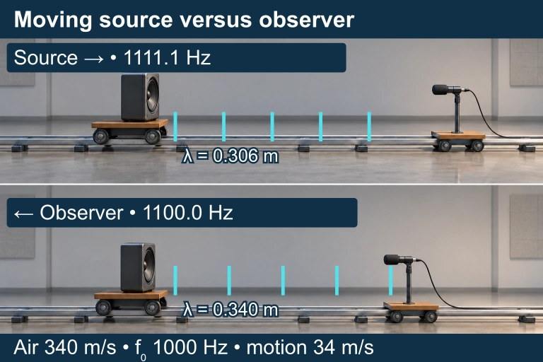At air speed 340 m/s and source 1000 Hz,34 m/s approaching source gives 1111.1 Hz and 0.306 m; approaching observer gives 1100 Hz with 0.340 m medium-frame wavelength. A source approaching a stationary observer compresses the wavelength; an approaching observer changes the encounter rate without changing medium-frame wavelength.

An ultrasound probe contacts gel on skin above a continuous vessel; an authored schematic shows incident/echo sound paths and a beam-flow calculation. A moving scatterer shifts the returning ultrasound frequency according to its velocity component along the beam. Motion away from the probe gives a negative echo shift; motion toward it gives a positive shift.

The echo shift depends on the velocity component along the beam.. A moving scatterer shifts the returning ultrasound frequency according to its velocity component along the beam. Motion away from the probe gives a negative echo shift; motion toward it gives a positive shift. 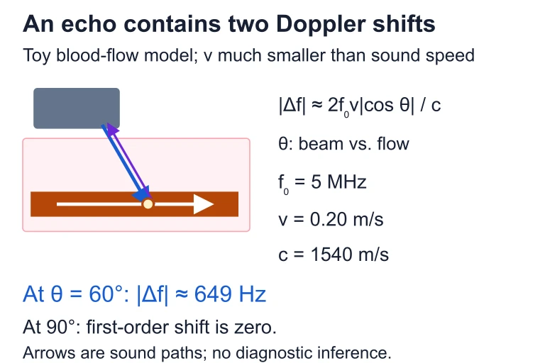A moving scatterer shifts the returning ultrasound frequency according to its velocity component along the beam. Motion away from the probe gives a negative echo shift; motion toward it gives a positive shift.

SECTION 6

Worked Example

Fire Truck Approaching and Receding

1
Step 1 — Identify Given Values

A fire truck siren emits sound at f₀ = 800 Hz. The truck moves at v_s = 30 m/s toward a stationary observer. The speed of sound in air is v = 343 m/s. We need to find the frequency heard by the observer as the truck (a) approaches and (b) recedes.
2
Step 2 — Choose the Correct Form of the Equation

Because the observer is stationary (v_o = 0), we use f = f₀ × v / (v ∓ v_s). For approach, subtract v_s in the denominator; for recession, add v_s.
3
Step 3 — Calculate Approaching Frequency

f_approach = 800 × 343 / (343 − 30) = 800 × 343 / 313 = 800 × 1.0959 ≈ 876.7 Hz.

f_approach ≈ 877 Hz
4
Step 4 — Calculate Receding Frequency

f_recede = 800 × 343 / (343 + 30) = 800 × 343 / 373 = 800 × 0.9196 ≈ 735.7 Hz.

f_recede ≈ 736 Hz
5
Step 5 — Interpret the Results

As the truck approaches, the observer hears a frequency about 77 Hz above the emitted tone—a noticeably higher pitch. After the truck passes and recedes, the frequency drops to about 64 Hz below the emitted tone. The total perceived shift as the truck passes is 877 − 736 ≈ 141 Hz, a dramatic change that matches everyday experience.

SECTION 7

Strengths, Limitations & Common Pitfalls

Strength	Limitation / Pitfall
Simple algebraic formula applicable to any sound-wave problem on the exam.	Only valid when both source and observer speeds are less than the wave speed (v_s < v). At v_s ≥ v, a shock wave (sonic boom) forms and the standard equation breaks down.
Qualitative reasoning (approach → higher f, recession → lower f) works for both sound and light.	The mechanical Doppler equation cannot be applied to light. Light requires the relativistic Doppler formula because there is no preferred medium.
Applies to any wave that travels through a medium: sound in air, water waves, seismic waves.	The equation assumes one-dimensional motion along the line connecting source and observer. Off-axis motion requires the cos θ correction factor.
Explains real-world phenomena students encounter daily (sirens, echoes, radar).	Students often confuse moving-source and moving-observer cases, applying signs incorrectly. Always check: does your answer predict a higher or lower frequency, and does that match the physical situation?

Strengths and limitations of the Doppler effect equations on the AP Physics 2 exam

🎯

EXAM STRATEGY

The single most common error on Doppler effect exam problems is a sign mistake. Before plugging in numbers, always perform a qualitative check: if the source and observer are closing in on each other, the observed frequency must be higher than f₀. If your math gives a lower value, you have a sign error. Think of it like proofreading: the physics must make sense before you trust the algebra.

SECTION 8

Connection to Advanced Theory

The mechanical Doppler equation you use in AP Physics 2 is the non-relativistic, one-dimensional form. In more advanced courses you will encounter extensions that broaden its scope. The relativistic Doppler effect for electromagnetic waves eliminates the medium dependence by incorporating time dilation from special relativity. The Mach number framework extends the analysis to supersonic sources, explaining shock cones and sonic booms. Finally, the cosmological redshift is conceptually related to the Doppler effect but arises from the expansion of space itself rather than from relative motion through a medium.

Feature	AP Physics 2 (Mechanical Doppler)	Advanced (Relativistic / Cosmological)
Wave type	Mechanical waves (sound, water)	Electromagnetic waves (light, radio)
Medium required?	Yes — v depends on the medium	No — light propagates through vacuum
Source vs. observer distinction?	Yes — the two cases yield different formulas	No — only relative velocity matters (Einstein's postulates)
Speed limit	v_s < v (subsonic only)	v < c (always satisfied for massive objects)
Key equation	f = f₀(v ± $v_o$ )/(v ∓ $v_s$ )	f = f₀ √[(1 ± β)/(1 ∓ β)], β = v/c

Comparison of the mechanical and relativistic Doppler frameworks

Recognizing where the AP-level formula ends and where advanced treatments begin will help you scope your answers on the exam. If a free-response question asks about the Doppler shift of light, provide a qualitative explanation (approach → blueshift, recession → redshift) without attempting to use the mechanical sound formula—examiners specifically look for this distinction.

SECTION 9

Practice Problems

Question 1: CONCEPTUAL

A train blowing its horn approaches a stationary observer, passes by, and then moves away. Which of the following best describes the frequency observed at each stage?

A. The observed frequency is higher than f₀ during approach, equals f₀ at the instant of passing, and is lower than f₀ during recession.
B. The observed frequency is lower than f₀ during approach and higher than f₀ during recession.
C. The observed frequency equals f₀ at all times because the wave speed in air is constant.
D. The observed frequency is higher than f₀ during both approach and recession because the source is in motion.

Show answer (A)

Choice A is correct. During approach, wavefronts are compressed in front of the source, so the observer detects a frequency higher than f₀. At the exact moment the source passes (radial velocity is zero), the observer momentarily hears f₀. During recession, wavefronts are stretched, and the observed frequency drops below f₀. Choice B reverses the shift directions, which contradicts the Doppler effect. Choice C ignores the effect entirely—while the wave speed is constant, the effective wavelength changes due to the source's motion. Choice D incorrectly suggests motion always raises frequency, but direction of motion matters.

Question 2: BASIC CALCULATION

A stationary speaker emits a 500 Hz tone. An observer drives toward the speaker at 25 m/s. The speed of sound is 343 m/s. What frequency does the observer hear?

A. 463 Hz
B. 500 Hz
C. 536 Hz
D. 540 Hz

Show answer (C)

With the source stationary (

v_s

= 0) and the observer moving toward the source, f = f₀ × (v +

v_o

) / v = 500 × (343 + 25) / 343 = 500 × 368 / 343 = 500 × 1.0729 ≈ 536 Hz. Choice A (463 Hz) would result from subtracting

v_o

in the numerator, as if the observer were moving away. Choice B (500 Hz) ignores the Doppler shift entirely. Choice D (540 Hz) could result from the moving-source formula, f = f₀ × v / (v −

v_s

), which is the wrong physical scenario. Choice C is correct.

Question 3: INTERMEDIATE

A car traveling at 35 m/s sounds its horn at 400 Hz. A cyclist rides toward the car at 10 m/s. If the speed of sound is 343 m/s, what frequency does the cyclist hear?

A. 446 Hz
B. 458 Hz
C. 465 Hz
D. 472 Hz

Show answer (B)

Both source and observer are moving toward each other. The observer (cyclist) moves toward the source, so add

v_o

to the numerator. The source (car) moves toward the observer, so subtract

v_s

from the denominator. f = 400 × (343 + 10) / (343 − 35) = 400 × 353 / 308 = 400 × 1.1461 ≈ 458 Hz. Choice A (446 Hz) could result from neglecting the cyclist's velocity. Choice C (465 Hz) and Choice D (472 Hz) likely result from sign errors or incorrect placement of velocities. Choice B is correct.

Question 4: APPLIED

5 pts

A student wants to experimentally verify the Doppler effect for sound using a battery-powered speaker mounted on a cart, a straight track, a microphone connected to a frequency analyzer, and a meterstick. (a) Describe a procedure the student could use to collect data that relates the speed of the source to the observed frequency. (b) Identify the independent and dependent variables. (c) Describe how the student should analyze the data to confirm the Doppler relationship. (d) State one assumption the student must make and explain how a violation of that assumption would affect the results. (e) Describe one modification to reduce systematic error in the experiment.

Show answer

Rubric (5 points): (1 pt) Procedure: The student sets the speaker to emit a known constant frequency f₀, places the microphone at one end of the track, and pushes the cart at different constant speeds toward the microphone. The cart's speed is measured by timing how long it takes to travel a measured distance (using the meterstick and a stopwatch or photogate). The frequency analyzer records the observed frequency f for each trial. (1 pt) Variables: The independent variable is the source speed

v_s

(varied by pushing the cart at different speeds). The dependent variable is the observed frequency f measured by the frequency analyzer. Controlled variables include the emitted frequency f₀, the temperature of the room (affecting v), and the position of the microphone. (1 pt) Data analysis: Plot f vs. 1/(v −

v_s

). According to f = f₀ × v / (v −

v_s

), a plot of f versus 1/(v −

v_s

) should be linear with slope f₀ × v and y-intercept zero. Alternatively, plot f vs.

v_s

and compare the shape to the theoretical curve. (1 pt) Assumption and violation: The student must assume the cart moves at constant speed during the measurement interval. If the cart accelerates or decelerates, the observed frequency will vary during a single trial, producing a spread of measured frequencies rather than a single value, introducing random error. (1 pt) Modification for systematic error: Use a longer track so that the cart can reach a steady speed before entering the measurement zone near the microphone. Alternatively, use photogates at two known positions to measure the cart's instantaneous speed more accurately than timing with a stopwatch.

Question 5: CRITICAL THINKING

4 pts

Two students debate whether the Doppler effect can change the speed of a sound wave. Student A claims that because the observed frequency changes, the wave speed must also change. Student B claims that the sound speed in the medium is fixed by its properties: source motion changes wavefront spacing in that frame, whereas observer motion changes encounter rate without changing that spacing. (a) Which student is correct? Justify your answer using the relationship v = fλ. (b) Explain physically why the wave speed does not depend on the motion of the source. (c) Suppose the observer moves toward a stationary source. Does the wave speed relative to the observer change? Explain. (d) Contrast this situation with the electromagnetic Doppler effect and explain why the mechanical Doppler formula cannot be used for light.

Show answer

Rubric (4 points): (1 pt) Part (a): Student B correctly distinguishes the medium frame from the moving observer's frame. For a stationary source, λmedium = v/f0. An observer approaching at speed vo measures fobs = (v + vo)/λmedium, so fobs λmedium = v + vo, not v. For a source approaching a stationary observer, λfront = (v − vs)/f0 and fobs = v/λfront. Thus v = fλ must use quantities belonging to the same frame and situation. (1 pt) Part (b): Each emitted wavefront propagates through the air at the speed fixed by the medium's properties. The source's subsequent motion changes where the next wavefront begins, not the speed of an already emitted wavefront. (1 pt) Part (c): The sound-wave speed relative to an approaching observer is v + vo. The observer meets fronts more rapidly, while the wave speed and front spacing measured in the medium's rest frame remain unchanged for a stationary source. (1 pt) Part (d): Light needs no material medium. All inertial observers measure its vacuum speed as c, so the mechanical formulas with a preferred medium frame do not apply. Relativistic Doppler relations account for relative motion and time dilation.

SUMMARY

Summary

The Doppler effect describes the change in observed frequency when a wave source and observer are in relative motion. For sound, the general equation is f = f₀(v ± $v_o$ )/(v ∓ $v_s$ ), where the sign choices are dictated by whether source and observer are approaching (higher f) or receding (lower f). The wave speed v is set by the medium and does not change with source or observer motion.

Key exam strategies: always perform a qualitative check on your answer (does the shift direction make physical sense?), distinguish between moving-source and moving-observer scenarios because they alter different parts of the equation, and remember that for electromagnetic waves only qualitative reasoning (blueshift vs. redshift) is expected on AP Physics 2. Applications range from medical Doppler ultrasound to astronomical redshift, demonstrating the far reach of a single wave-propagation principle.