Electric Potential - AP Physics 2

SECTION 1

Historical Context & Motivation

The concept of electric potential arose from the need to describe electrical phenomena without tracking the detailed motion of every individual charge. In the eighteenth and nineteenth centuries, experimenters observed that charged objects stored a capacity for doing work and that the "electrical condition" of a point in space could be characterized independently of any particular test charge placed there. This insight—that the field itself carries energetic information—transformed electrostatics from a catalog of force measurements into a predictive framework capable of guiding the design of circuits, capacitors, and eventually the electrical grid that powers modern civilization.

1745 • The Leyden Jar

Pieter van Musschenbroek and Ewald Georg von Kleist independently invent the Leyden jar, demonstrating that electric charge can be stored and later released to do work—an early, tangible encounter with electric potential energy.

1785 • Coulomb's Law

Charles-Augustin de Coulomb publishes precise force measurements using a torsion balance, establishing the inverse-square law for electrostatic force and providing the quantitative foundation for defining potential energy between point charges.

1800 • The Voltaic Pile

Alessandro Volta constructs the first true battery, maintaining a steady potential difference between its terminals and launching the study of continuous current. The unit of electric potential—the volt—is named in his honor.

1828 • Green's Mathematical Theory

George Green introduces the concept of a potential function in his essay on electricity and magnetism, formalizing the scalar field whose gradient yields the electric field vector—bridging force and energy descriptions.

1867 • Thomson & Maxwell's Field Theory

Lord Kelvin and James Clerk Maxwell embed electric potential firmly within the mathematical structure of classical field theory, showing that equipotential surfaces and field lines together provide a complete geometric picture of electrostatics.

The central question these developments converge on is deceptively simple: How much work does the electric field do—or how much energy must an external agent supply—when a charge moves from one location to another? Answering this question with a scalar quantity, rather than by integrating vector forces along every conceivable path, is exactly the power that electric potential provides. The remainder of this lesson develops that idea rigorously, equipping you with the conceptual and mathematical tools the AP Physics 2 exam demands.

SECTION 2

Core Principles & Definitions

Electric potential is fundamentally an energy-per-charge quantity. It assigns a single number—a scalar—to every point in space surrounding a charge distribution, capturing all the information needed to determine how much work the electric field performs on any charge that moves through it. Because it is a scalar rather than a vector, electric potential is often far easier to work with than the electric field when solving for energy changes, voltage differences across circuit elements, or the behavior of charges near conductors. The following grid lays out the five foundational ideas that anchor the concept.

Electric Potential (V)

The electric potential at a point is defined as the electric potential energy per unit positive test charge at that point: V = U_E / q. Its SI unit is the volt (1 V = 1 J / C).

Potential Difference (ΔV)

Only differences in potential are physically measurable. The potential difference between two points, ΔV = V_B − V_A, determines the work done per unit charge by the field when a charge moves from A to B.

Scalar Superposition

Because potential is a scalar, the net potential at any point due to multiple source charges is the algebraic sum of the individual potentials—no vector components to resolve. This makes calculations dramatically simpler than summing electric field vectors.

Equipotential Surfaces

Equipotential surfaces connect points of equal potential. No work is done when a charge moves along an equipotential. These surfaces are always perpendicular to the electric field lines.

Relationship to Electric Field

The electric field points in the direction of decreasing potential. In a uniform field, E = −ΔV / Δd, linking the field strength to how rapidly the potential changes with position.

✦

KEY TAKEAWAY

Think of electric potential as the electrical altitude of a point in space. Just as a topographic map shows gravitational altitude without specifying whether a hiker, a boulder, or a bicycle sits at each point, the electric potential map describes the energy landscape without reference to any particular charge. A positive charge naturally "rolls downhill" from high potential to low potential, just as water flows from high elevation to low elevation. The steeper the slope (the greater the rate at which potential changes with distance), the stronger the electric field at that location.

SECTION 3

Equipotential Lines & Field Lines

A powerful way to build intuition about electric potential is to visualize equipotential lines alongside electric field lines. The diagram below depicts a positive point charge at the center. The concentric circles are equipotential lines—every point on a given circle has the same potential value. The radial arrows are electric field lines, pointing outward (the direction a positive test charge would accelerate). Notice that the two families of curves are everywhere perpendicular, a geometric fact that holds for any charge distribution, not just the symmetric case shown here.

The dashed cyan circles are equipotential lines at successively lower potentials as the distance from the positive source charge increases. The solid violet arrows are electric field lines, always perpendicular to the equipotentials and pointing from high to low potential.

Several features of the diagram deserve emphasis. First, the equipotential lines are more closely spaced near the charge, reflecting the fact that the potential changes more rapidly there—this corresponds to a stronger electric field. Second, a test charge moving along any one of those cyan circles does so at constant potential, meaning the electric field does zero work on it during such motion. Third, the potential values decrease as 1/r (shown by the labeled values), which is a direct consequence of Coulomb's law applied to a point charge. These geometric relationships generalize: for any charge distribution, the electric field is always perpendicular to equipotential surfaces, and closely spaced equipotentials signal a strong field.

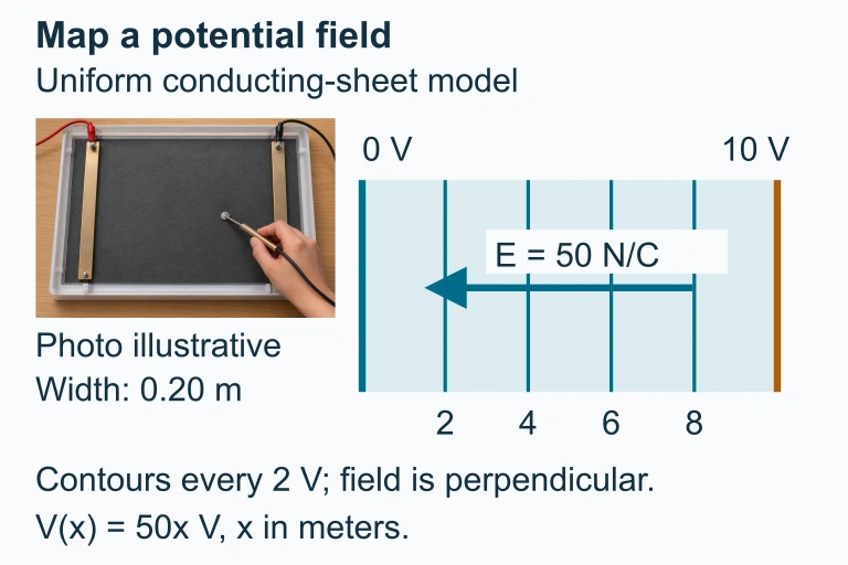Conducting sheet V(x)=50 x, span 0.2 m and 0→10 V; E=−50 x-hat N/C perpendicular to equipotentials. In this selected synthetic sheet model, equal potential increments form evenly spaced contours and the electric field points toward lower potential.

SECTION 4

Mathematical Framework

The mathematical description of electric potential connects several core ideas: the definition of potential in terms of work or energy, the potential due to a point charge, the superposition principle for multiple charges, and the relationship between potential and the electric field. Each of these equations appears regularly on the AP Physics 2 exam, so fluency with their meaning, units, and applicability is essential.

DEFINITION OF ELECTRIC POTENTIAL

V = U_E / q

V = electric potential (volts, V), U_E = electric potential energy (joules, J), q = charge of the test object (coulombs, C). A potential of 1 volt means 1 joule of potential energy per coulomb of charge.

POTENTIAL DUE TO A POINT CHARGE

V = kQ / r

k = Coulomb's constant ≈ 8.99 × 10⁹ N·m²/C², Q = source charge (C), r = distance from the source charge (m). This potential is measured relative to V = 0 at infinity. Note that V is positive for a positive source charge and negative for a negative source charge—the sign of Q matters.

SUPERPOSITION OF POTENTIALS

V_net = V₁ + V₂ + V₃ + … = k Σ (Qᵢ / rᵢ)

Because potential is a scalar, the total potential at a point is the algebraic (signed) sum of the individual potentials from each source charge. There is no need to decompose into x- and y-components.

RELATIONSHIP BETWEEN FIELD AND POTENTIAL (UNIFORM FIELD)

ΔV = −E · Δd

E = magnitude of the uniform electric field (V/m or N/C), Δd = displacement in the direction of the field (m). The negative sign encodes the fact that the field points from high potential to low potential. For a uniform field between parallel plates, E = |ΔV| / d, where d is the plate separation.

⚠

Sign Conventions Matter

A common exam pitfall is dropping the sign of the source charge Q in V = kQ/r. The potential due to a negative charge is itself negative, even though distance r is always positive. When using superposition, include the sign of each Q; cancellation between positive and negative terms is expected and physically meaningful. Similarly, ΔV = V_final − V_initial; reversing the order flips the sign of the work done by the field.

SECTION 5

Electric Potential Energy & Charge Motion

While electric potential describes the energy landscape of space itself, electric potential energy describes the energy that a specific charge possesses by virtue of its position within that landscape. The relationship is straightforward—U_E = qV—but the implications are profound. A positive charge released from rest accelerates toward lower potential (gaining kinetic energy and losing potential energy), while a negative charge accelerates toward higher potential. This directional difference is the core reason that conventional current flows from high to low potential in circuits, whereas electrons physically drift the other way.

Between uniformly charged parallel plates, the electric field is uniform and points from the positive plate (high V) to the negative plate (low V). A positive charge accelerates in the direction of E (toward lower V), while a negative charge accelerates opposite to E (toward higher V). Both gain kinetic energy at the expense of electric potential energy.

The connection between potential difference and kinetic energy is captured by the work-energy theorem applied to electric forces: W_field = qΔV = ΔKE. For a charge released from rest, this becomes ½mv² = |q||ΔV|. This equation is the basis of particle accelerators and is tested frequently in AP contexts involving charges moving through known potential differences. It is also the origin of the electron-volt (eV), a convenient energy unit defined as the kinetic energy gained by one elementary charge accelerated through a potential difference of 1 volt: 1 eV = 1.6 × 10⁻¹⁹ J.

Charge Sign	Moves Toward	ΔV Along Path	Δ $U_E$	ΔKE
Positive (+q)	Lower V	Negative (V decreases)	Decreases	Increases
Negative (−q)	Higher V	Positive (V increases)	Decreases	Increases

Both positive and negative charges lose potential energy and gain kinetic energy when released in a field; they simply move in opposite directions.

SECTION 6

Worked Example: Potential & Speed of a Proton

A proton is released from rest near the positive plate of a parallel-plate capacitor. The plates are separated by 2.0 cm and the potential difference across the plates is 150 V. Determine (a) the electric field between the plates, (b) the change in potential energy of the proton as it crosses from the positive plate to the negative plate, and (c) the speed of the proton when it reaches the negative plate. (m_p = 1.67 × 10⁻²⁷ kg, e = 1.60 × 10⁻¹⁹ C.)

Proton Between Parallel Plates

1
Step 1 — Identify Given Values

Plate separation d = 2.0 cm = 0.020 m. Potential difference |ΔV| = 150 V. The proton has charge q = +1.60 × 10⁻¹⁹ C and mass m_p = 1.67 × 10⁻²⁷ kg. It starts from rest, so v₀ = 0.
2
Step 2 — Calculate the Electric Field (Part a)

For a uniform field between parallel plates, E = |ΔV| / d = 150 V / 0.020 m.

E = 7500 V/m = 7.5 × 10³ N/C
3
Step 3 — Find the Change in Potential Energy (Part b)

The proton moves from the positive plate (high V) to the negative plate (low V), so ΔV = V_final − V_initial = −150 V. The change in potential energy is ΔU_E = qΔV = (1.60 × 10⁻¹⁹ C)(−150 V).

Δ $U_E$ = −2.40 × 10⁻¹⁷ J (The negative sign confirms the proton loses potential energy.)
4
Step 4 — Apply Conservation of Energy (Part c)

Since the proton starts from rest, all lost potential energy converts to kinetic energy: ½m_pv² = |ΔU_E| = 2.40 × 10⁻¹⁷ J. Solving for v: v = √(2 × 2.40 × 10⁻¹⁷ / 1.67 × 10⁻²⁷).

v ≈ 1.70 × 10⁵ m/s
5
Step 5 — Check Reasonableness

This speed is about 0.06% of the speed of light, so non-relativistic treatment is valid. The proton moves toward lower potential (as expected for a positive charge), and its kinetic energy gain equals 150 eV—consistent with the 150 V potential difference.

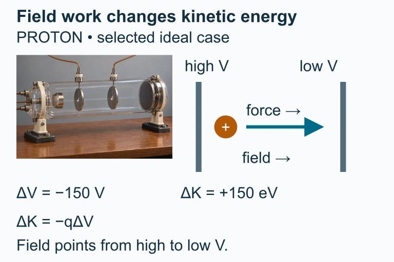Positive proton from +150 V to 0 V gains 150 eV; force and E agree. Separate proton case with a 150 V potential drop.

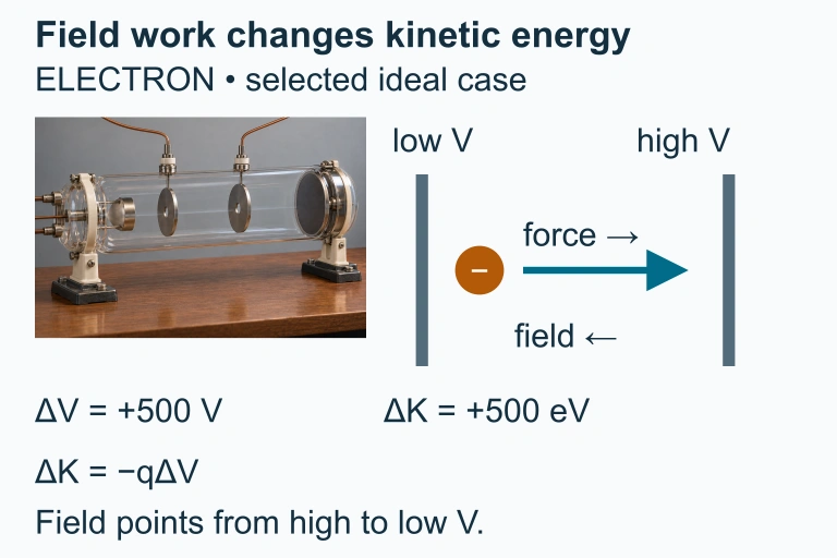Electron gains 500 eV moving from 0 to +500 V, opposite E, with force opposite E. Electron case: reverse field polarity for acceleration to the right.

SECTION 7

Potential vs. Electric Field: Strengths & Limitations

Students often wonder: if the electric field already tells us the force on a charge, why introduce electric potential at all? The answer lies in computational convenience and physical insight. Each representation—field or potential—excels in different problem types. The table below compares the two quantities across several important dimensions, helping you decide which tool to reach for on a given problem.

Feature	Electric Field (E)	Electric Potential (V)
Type	Vector (magnitude and direction)	Scalar (magnitude and sign only)
SI Unit	N/C (or V/m)	V (volt = J/C)
Superposition	Vector addition (must resolve components)	Algebraic addition (just add signed numbers)
Best For	Finding force on a charge, direction of motion	Finding energy changes, voltage in circuits, superposition of many charges
Measured By	Test charge and force probe	Voltmeter
Limitation	Component calculations become complex for many sources	Only differences are measurable; does not directly give force direction

Comparison of electric field and electric potential as problem-solving tools.

✦

KEY TAKEAWAY

Electric field and electric potential are two complementary views of the same physical reality, much like how a topographic map (potential) and a slope/gradient map (field) describe the same mountain. Engineers designing circuits almost always work with potential (voltage), while physicists analyzing particle trajectories often prefer the field. Mastering both representations—and knowing when each is more efficient—is a hallmark of strong physical reasoning.

SECTION 8

Connection to Advanced Theory

The electric potential you study in AP Physics 2 is actually a special case of more general frameworks in electromagnetism and beyond. In a university-level course, you will encounter the gradient operator (∇), which provides the precise mathematical link between the electric field vector and the potential scalar field in three dimensions: E⃗ = −∇V. This replaces the one-dimensional ΔV = −EΔd with a fully three-dimensional relationship. You will also encounter Laplace's and Poisson's equations, which govern how potential distributes itself in regions of space with and without charge, forming the backbone of computational electromagnetics.

Concept	AP Physics 2 Treatment	Advanced / University Treatment
E–V Relationship	ΔV = −EΔd for uniform fields; qualitative for non-uniform	E⃗ = −∇V (gradient operator in 3D, including curvilinear coordinates)
Superposition	Discrete sum: V = kΣ(Qᵢ/rᵢ)	Continuous integration: V(r) = k ∫ dq / \|r − r'\|
Boundary Conditions	Conductors are equipotential surfaces; V = 0 at infinity	Dirichlet & Neumann boundary conditions; uniqueness theorems
Time Dependence	Static (electrostatic) potential only	Scalar & vector potentials (V, A⃗) unify into the four-potential in special relativity

How electric potential concepts deepen at the university level.

Even within the AP course, these advanced ideas cast a useful shadow. Knowing that E⃗ is the gradient of V helps you reason qualitatively: where equipotential lines are tightly packed, the field is strong; where they are widely spaced, the field is weak. And the concept of a scalar potential extends directly to gravitational potential (V_g = −GM/r), so the intuition you build here transfers immediately to astrophysics and orbital mechanics.

SECTION 9

Practice Problems

Question 1: CONCEPTUAL

A positive charge is placed at a point where the electric potential is +50 V, and it is then moved to a point where the potential is +20 V. Which of the following correctly describes the work done by the electric field and the change in the charge's kinetic energy (assuming no other forces act)?

A. The electric field does negative work; the kinetic energy decreases.
B. The electric field does positive work; the kinetic energy increases.
C. The electric field does zero work; the kinetic energy is unchanged.
D. The electric field does positive work; the kinetic energy decreases.

Show answer (B)

B is correct. The work done by the electric field on a charge q moving through a potential difference is W = −qΔV = −q(V_f − V_i) = −q(20 − 50) = −q(−30) = +30q. Since q > 0, the field does positive work, which by the work-energy theorem increases kinetic energy. A is wrong because the charge moves to lower potential, so the field does positive (not negative) work. C is wrong because there is a 30 V potential difference—the work is nonzero. D is wrong because positive work by the net force must increase (not decrease) kinetic energy.

Question 2: BASIC CALCULATION

Two point charges, Q₁ = +3.0 μC and Q₂ = −5.0 μC, are separated by 0.40 m. What is the electric potential at the midpoint between them? (k = 8.99 × 10⁹ N·m²/C²)

A. −9.0 × 10⁴ V
B. +9.0 × 10⁴ V
C. −3.6 × 10⁵ V
D. +3.6 × 10⁵ V

Show answer (A)

A is correct. At the midpoint, r₁ = r₂ = 0.20 m. Using scalar superposition: V = kQ₁/r₁ + kQ₂/r₂ = (8.99 × 10⁹)(3.0 × 10⁻⁶)/(0.20) + (8.99 × 10⁹)(−5.0 × 10⁻⁶)/(0.20) = 1.35 × 10⁵ + (−2.25 × 10⁵) = −9.0 × 10⁴ V. B is wrong because it neglects the negative sign of Q₂ and would require the negative charge to contribute positive potential. C is wrong because it uses the full separation (0.40 m) instead of the midpoint distance (0.20 m), then misapplies superposition. D is wrong because it incorrectly reverses the sign and uses the wrong distance.

Question 3: INTERMEDIATE

An electron is accelerated from rest through a potential difference of 500 V. What is the final speed of the electron? (m_e = 9.11 × 10⁻³¹ kg, e = 1.60 × 10⁻¹⁹ C)

A. 4.2 × 10⁵ m/s
B. 1.33 × 10⁷ m/s
C. 1.87 × 10⁷ m/s
D. 6.63 × 10⁶ m/s

Show answer (B)

B is correct. The electron gains kinetic energy equal to the magnitude of its charge times the potential difference: ½m_ev² = eΔV = (1.60 × 10⁻¹⁹)(500) = 8.0 × 10⁻¹⁷ J. Solving: v = √(2 × 8.0 × 10⁻¹⁷ / 9.11 × 10⁻³¹) = √(1.76 × 10¹⁴) ≈ 1.33 × 10⁷ m/s. A is wrong because it appears to use the proton mass instead of the electron mass. C is wrong because it likely arises from an arithmetic error (forgetting the factor of 2 under the square root). D is wrong because it corresponds to using ΔV = 250 V (half the actual value), or equivalently omitting the factor of 2 in the energy equation.

Question 4: APPLIED

4 pts

A student has access to a DC power supply (0–30 V), two flat metal plates that can be held parallel, a ruler, a voltmeter with a probe, graph paper, and connecting wires. Design an experiment to verify the relationship E = |ΔV| / d for a uniform electric field between parallel plates. (a) Describe the experimental procedure, including what quantities are measured and how. (2 pts) (b) Describe how the student should analyze the collected data to verify the relationship. Include what should be graphed on each axis and what the expected result of the graph is if the relationship is valid. (1 pt) (c) Identify one source of systematic error in the experiment and explain the direction in which it would affect the measured value of the electric field. (1 pt)

Show answer

Rubric (4 points): Point 1 (Procedure — setup): Mount the two parallel plates vertically at a fixed, measured separation d. Connect the plates to the DC power supply, setting a known voltage ΔV. Use the voltmeter probe to measure the potential at several equally spaced positions between the plates along a line perpendicular to the plates. Point 2 (Procedure — variation): Repeat the measurements for at least four different plate separations d while keeping ΔV constant (or vary ΔV while keeping d constant). Record all distances with the ruler and all voltage readings with the voltmeter. Point 3 (Data analysis): If ΔV is held constant and d is varied, graph ΔV/d (calculated E) on the vertical axis versus 1/d on the horizontal axis. If E = |ΔV|/d is valid, the graph should be linear through the origin with slope equal to ΔV. Alternatively, if d is fixed and ΔV is varied, graph the measured potential at intermediate points as a function of position; a linear relationship confirms a uniform field with slope equal to E. Point 4 (Systematic error): Fringe effects (non-uniform field near the plate edges) constitute a systematic error. The field near the edges is weaker and non-uniform, so voltage measurements taken near the edges would indicate a weaker-than-expected field, causing the measured E to be systematically lower than ΔV/d. This can be mitigated by making measurements only near the center of the plates and by using plates whose area is much larger than d².

Question 5: CRITICAL THINKING

4 pts

Three point charges are arranged at the vertices of an equilateral triangle with side length a = 0.30 m. Two vertices carry charges of +4.0 μC each, and the third vertex carries a charge of −4.0 μC. (a) Determine the electric potential at the center of the triangle. (2 pts) (b) A proton is placed at the center of the triangle and released from rest. Will it initially move toward the negative charge, away from the negative charge, or remain stationary? Justify your answer using the concepts of electric field and/or electric potential. (2 pts)

Show answer

Rubric (4 points): Point 1 (Part a — distance to center): The distance from each vertex to the centroid of an equilateral triangle is r = a/√3 = 0.30/√3 ≈ 0.173 m. Point 2 (Part a — superposition): Electric potential is a scalar, so V = k(Q₁ + Q₂ + Q₃)/r = (8.99 × 10⁹)[(+4.0 × 10⁻⁶) + (+4.0 × 10⁻⁶) + (−4.0 × 10⁻⁶)] / 0.173 = (8.99 × 10⁹)(4.0 × 10⁻⁶) / 0.173 ≈ 2.1 × 10⁵ V. The net electric potential at the center is approximately +2.1 × 10⁵ V. Point 3 (Part b — direction of motion): The proton initially accelerates toward the negative charge. The direction of motion is determined by the electric field (a vector), not the electric potential (a scalar). By symmetry, the electric field contributions from the two +4.0 μC charges at the center partially cancel in the direction parallel to the line joining them, but their components pointing away from the positive-charge side add together. The field from the −4.0 μC charge points toward it. The resultant net electric field at the center points from the midpoint of the two positive charges toward the negative charge. Since a proton is positive, it accelerates in the direction of the net electric field—toward the negative charge. Point 4 (Part b — justification distinguishing field from potential): The student must clearly state that although the electric potential at the center is nonzero, potential is a scalar and does not indicate direction. The electric field is a vector quantity that determines the force on the proton and thus its direction of acceleration. A nonzero potential does not imply the proton remains stationary; the nonzero net electric field at the center is what causes the proton to accelerate toward the negative charge.

SUMMARY

Summary & Key Concepts

Summary

Electric potential (V) assigns a scalar value to every point in space, representing the electric potential energy per unit charge at that location. The potential due to a point charge is V = kQ/r, and the total potential from multiple charges is found by scalar superposition—simply adding signed values without resolving vector components. Only potential differences (ΔV) are physically measurable, and they determine the work done by the electric field on moving charges: W = −qΔV.

Equipotential surfaces are always perpendicular to electric field lines, and the field points from high to low potential. In a uniform field between parallel plates, the relationship simplifies to E = |ΔV|/d. A charge accelerated through a potential difference gains kinetic energy ½mv² = |q||ΔV|, a principle that underlies particle accelerators and defines the electron-volt energy unit. Mastering both the scalar (potential) and vector (field) descriptions—and knowing when each is the more efficient tool—is essential for success on the AP Physics 2 exam.