Electric Fields - AP Physics 2

SECTION 1

Historical Context & Motivation

The notion that charged objects can influence one another across empty space posed one of the deepest puzzles in the history of physics. In the eighteenth century, Charles-Augustin de Coulomb quantified the force between point charges and demonstrated that it obeys an inverse-square law, much like gravity. Yet a fundamental question remained: how does one charge "know" the other is there? The concept of action at a distance troubled physicists, because it implied instantaneous influence with no mediating mechanism. It was Michael Faraday's revolutionary insight — that charged bodies create an invisible field pervading the surrounding space — that shifted the paradigm from forces acting at a distance to a local field-based description of electromagnetic phenomena.

1785 • Coulomb's Torsion-Balance Experiments

Coulomb publishes precise measurements confirming that the electric force between two point charges varies as the inverse square of the distance and is proportional to the product of the charges.

1831 • Faraday Introduces "Lines of Force"

Michael Faraday visualizes the space around charged objects as filled with curved lines of force, laying the conceptual groundwork for the electric field. His intuitive geometric picture remains central to physics education today.

1862 • Maxwell's Field Equations

James Clerk Maxwell translates Faraday's qualitative field picture into a rigorous mathematical framework — a set of differential equations that unify electricity and magnetism and predict electromagnetic waves.

1909 • Millikan's Oil-Drop Experiment

Robert Millikan measures the fundamental unit of electric charge using an electric field to suspend tiny oil droplets, confirming that charge is quantized and providing a precise value of e.

The central question this lesson addresses is both conceptual and practical: How do we describe the influence a charged object exerts on the space around it, and how can we use that description to predict the force on any other charge placed in that region? By introducing the electric field as an independent physical quantity defined at every point in space, we gain a tool that is far more powerful and general than simply cataloging forces between pairs of charges.

SECTION 2

Core Principles & Definitions

An electric field is a vector quantity that exists at every point in the space surrounding a charged object (the source charge). Operationally, the field at a given location is defined as the electric force per unit positive charge that would be experienced by a small test charge placed there. Crucially, the test charge must be small enough that it does not significantly disturb the source charge distribution. Because the field is a property of the space itself — created by the source — it exists whether or not a test charge is actually present. This is the conceptual leap Faraday made: the field is real, not merely a mathematical convenience.

Electric Field as Force per Charge

The electric field E⃗ at a point equals the force F⃗ that would act on a positive test charge q₀ divided by q₀. Its SI unit is newtons per coulomb (N/C), equivalently volts per meter (V/m).

Direction Convention

The electric field points in the direction of the force on a positive test charge. Field lines radiate outward from positive source charges and inward toward negative source charges.

Superposition Principle

When multiple source charges are present, the total electric field at any point is the vector sum of the fields produced by each individual charge. This linearity is fundamental and allows complex configurations to be analyzed piece by piece.

Field Lines

Electric field lines are visual tools. They begin on positive charges and end on negative charges (or extend to infinity). The density of lines in a region represents the field magnitude, and the tangent to a line at any point gives the field direction.

✦

KEY TAKEAWAY

Think of the electric field like a weather map for electric force. A weather map assigns a wind vector to every location — speed and direction — so that a pilot can predict the force the air will exert on an airplane anywhere on the map. Likewise, the electric field assigns a force-per-charge vector to every point in space. Once the "map" is established by the source charges, you can instantly predict the force on any charge placed anywhere in the region, simply by multiplying: F⃗ = qE⃗.

SECTION 3

Visualizing Electric Fields

Electric field lines provide one of the most powerful ways to build intuition about the behavior of electric fields. The following diagram illustrates the field line patterns for three foundational configurations: a single positive point charge, a single negative point charge, and an electric dipole (a pair of equal-magnitude but opposite charges). Observe how the density and curvature of the lines encode both the magnitude and direction of the field everywhere in the surrounding space.

Figure 1. Electric field line patterns for three fundamental configurations. Left: A positive point charge — lines radiate outward symmetrically. Center: A negative point charge — lines point inward. Right: An electric dipole — field lines curve from the positive charge to the negative charge, illustrating how the fields of the two charges superpose.

Several key features of the diagram deserve attention. For the isolated positive charge on the left, the lines are symmetric and radial; their spacing increases with distance from the charge, reflecting the inverse-square decrease in field magnitude. For the negative charge in the center, the pattern is identical in shape but the arrows point inward, toward the charge. In the dipole configuration on the right, the lines originate on the positive charge and terminate on the negative charge, curving outward and back. Between the charges the field is strong (lines are dense), while far from the dipole the lines become sparse and the configuration increasingly resembles that of a neutral object. Note that field lines never cross — because the electric field has a unique direction at every point, two lines intersecting would imply two different directions, which is physically impossible.

SECTION 4

Mathematical Framework

The quantitative treatment of electric fields connects the conceptual field picture to measurable, calculable quantities. We begin with the operational definition of the electric field, then specialize to the important case of the field produced by a point charge, and finally state the superposition principle in mathematical form.

DEFINITION OF ELECTRIC FIELD

E⃗ = F⃗ / q₀

E⃗ = electric field vector (N/C or V/m); F⃗ = electrostatic force on the test charge (N); q₀ = positive test charge (C). The test charge must be vanishingly small so as not to perturb the source distribution.

FIELD OF A POINT CHARGE

E = kQ / r²

k = Coulomb's constant ≈ 8.99 × 10⁹ N·m²/C²; Q = source charge (C); r = distance from the source charge to the field point (m). The field points radially outward if Q > 0 and radially inward if Q < 0.

SUPERPOSITION OF FIELDS

E⃗_net = E⃗₁ + E⃗₂ + E⃗₃ + ⋯ = Σ E⃗ᵢ

The net electric field at any point is the vector sum of the fields produced by each individual source charge. Because this is a vector addition, you must resolve components along orthogonal axes and sum them separately before recombining.

FORCE ON A CHARGE IN AN EXTERNAL FIELD

F⃗ = qE⃗

Once the electric field is known, the force on any charge q placed in that field is simply the charge multiplied by the field vector. If q is negative, the force is opposite to the field direction.

💡

AP Exam Tip

On the AP Physics 2 exam, you will frequently need to find the electric field at a point due to two or more charges. Remember to break each field vector into x- and y-components, sum the components separately (E_x,net = ΣE_x,i and E_y,net = ΣE_y,i), and then find the magnitude and direction of the resultant. Sketching a diagram first is essential for getting signs and angles correct.

SECTION 5

Common Field Configurations

Beyond isolated point charges, the AP Physics 2 curriculum requires familiarity with the electric field patterns of several common charge configurations. Understanding these canonical cases — the uniform field between parallel plates, the radial field of a charged sphere, and the field of continuous charge distributions — builds the physical intuition needed to analyze more complex scenarios. The diagram below depicts the uniform field between two large parallel conducting plates, one of the most frequently tested setups on the exam.

Figure 2. A uniform electric field exists between two large, parallel conducting plates carrying equal and opposite charges. The field lines are parallel, equally spaced, and directed from the positive plate to the negative plate, indicating a constant field magnitude throughout the interior. A positive test charge q (green) experiences a force F⃗ = qE⃗ in the direction of the field.

Configuration	Field Magnitude	Key Feature
Point Charge	E = kQ / r²	Radial symmetry; decreases with inverse square of distance
Parallel Plates	E = V / d = σ / ε₀	Uniform field between plates; E is independent of position
Conducting Sphere (outside)	E = kQ / r² (r > R)	Behaves as if all charge were at center; zero field inside
Insulating Sphere (inside)	E = kQr / R³ (r < R)	Field increases linearly with r for uniform charge density

Table 1. Summary of electric field expressions for common charge configurations tested on AP Physics 2.

The parallel-plate configuration is especially important because it produces a uniform electric field — one whose magnitude and direction are the same everywhere between the plates (neglecting edge effects). This simplification makes it the go-to setup for problems involving charged-particle motion, energy arguments, and connections to electric potential. The relationship E = V/d, where V is the potential difference between the plates and d is the plate separation, appears repeatedly on both the multiple-choice and free-response sections of the AP exam.

SECTION 6

Worked Example: Superposition of Two Point Charges

Consider two point charges arranged along the x-axis. Charge q₁ = +4.0 μC is located at the origin, and charge q₂ = −9.0 μC is located at x = 0.30 m. We wish to find the net electric field at point P, located on the x-axis at x = 0.10 m (between the two charges).

Net Electric Field at Point P

1
Step 1 — Identify given values and geometry

q₁ = +4.0 × 10⁻⁶ C at x = 0. q₂ = −9.0 × 10⁻⁶ C at x = 0.30 m. Point P is at x = 0.10 m. The distance from q₁ to P is r₁ = 0.10 m. The distance from q₂ to P is r₂ = 0.30 − 0.10 = 0.20 m. Coulomb's constant k = 8.99 × 10⁹ N·m²/C².
2
Step 2 — Calculate the magnitude of E⃗₁ at P

Using E = kQ / r², we find E₁ = (8.99 × 10⁹)(4.0 × 10⁻⁶) / (0.10)² = (8.99 × 10⁹)(4.0 × 10⁻⁶) / 0.01.

E₁ = 3.60 × 10⁶ N/C
3
Step 3 — Determine the direction of E⃗₁ at P

Since q₁ is positive, the field it produces at P points away from q₁ — that is, in the +x direction.
4
Step 4 — Calculate the magnitude of E⃗₂ at P

E₂ = (8.99 × 10⁹)(9.0 × 10⁻⁶) / (0.20)² = (8.99 × 10⁹)(9.0 × 10⁻⁶) / 0.04.

E₂ = 2.02 × 10⁶ N/C
5
Step 5 — Determine the direction of E⃗₂ at P

Since q₂ is negative, the field it produces at P points toward q₂ — that is, in the +x direction (P is to the left of q₂, and the field points from P toward the negative charge).
6
Step 6 — Apply superposition

Both E⃗₁ and E⃗₂ point in the +x direction at P. Therefore E_net = E₁ + E₂ = 3.60 × 10⁶ + 2.02 × 10⁶.

E_net = 5.62 × 10⁶ N/C in the +x direction

⚠

Why Both Fields Point the Same Way

This is a common source of error. At point P, which lies between the two charges, E⃗₁ points away from the positive charge (to the right) while E⃗₂ points toward the negative charge (also to the right). When a positive and a negative charge are on opposite sides of a point, their fields at that point add rather than cancel. If both charges had been positive, the fields at an interior point would have pointed in opposite directions.

SECTION 7

Electric Field vs. Gravitational Field

Drawing explicit comparisons between the electric field and the gravitational field deepens understanding of both concepts. Both fields obey inverse-square laws for point-like sources, and both can be described using a field model that eliminates the need for action at a distance. However, significant differences exist — most notably that electric charge comes in two signs (producing both attractive and repulsive interactions) while gravitational mass is always positive (gravity is purely attractive). The table below highlights the most instructive parallels and contrasts.

Feature	Electric Field	Gravitational Field
Source	Electric charge (positive or negative)	Mass (always positive)
Force Law	F = kq₁q₂ / r² (Coulomb's law)	F = Gm₁m₂ / r² (Newton's law of gravitation)
Field Definition	E⃗ = F⃗ / q₀ (force per unit positive charge)	g⃗ = F⃗ / m₀ (force per unit mass)
Nature of Force	Attractive or repulsive (depends on sign of charges)	Always attractive
Relative Strength	Enormously stronger — dominates at atomic and molecular scales	Extremely weak — only significant for large (planetary-scale) masses
Shielding	Possible with conductors (Faraday cage)	Not possible — no known gravitational shielding

Table 2. Parallel structure of the electric and gravitational fields.

✦

KEY TAKEAWAY

The mathematical parallel between E⃗ = F⃗/q₀ and g⃗ = F⃗/m₀ is not a coincidence — it reflects a deep structural similarity in how physics describes fields. Mastering the concept of the electric field will pay dividends when you encounter magnetic fields, and eventually the idea of a field becomes the unifying language of modern physics, from electromagnetism to general relativity to quantum field theory.

SECTION 8

Connection to Electric Potential & Gauss's Law

The electric field does not exist in isolation within the theoretical framework of electromagnetism; it connects intimately to other key quantities you will encounter in AP Physics 2 and beyond. Two of the most important connections are to electric potential (voltage) and to Gauss's law. Understanding how the electric field relates to these concepts transforms the field from a standalone idea into a node in a rich conceptual network.

Concept	Relationship to Electric Field	Why It Matters
Electric Potential (V)	E = −ΔV / Δx (uniform field); the field points from high potential to low potential	Allows energy-based analysis; potential is a scalar (easier to sum than vectors)
Gauss's Law	Φ_E = ∮E⃗ · dA⃗ = Q_enc / ε₀	Relates the total electric flux through a closed surface to the enclosed charge; powerful for symmetric geometries
Equipotential Surfaces	E⃗ is always perpendicular to equipotential surfaces	Visual tool for mapping fields; no work is done moving a charge along an equipotential
Conductors in Equilibrium	E⃗ = 0 inside; E⃗ is perpendicular to the surface outside	Explains shielding, charge redistribution, and the behavior of Faraday cages

Table 3. How the electric field connects to other key topics in electrostatics.

Looking forward, the field concept extends naturally to time-varying situations: a changing magnetic field produces an electric field (Faraday's law of induction), and a changing electric field produces a magnetic field (Ampère–Maxwell law). Together, these relationships form the backbone of Maxwell's equations, which unify all of classical electromagnetism and predict the existence of electromagnetic waves. The static electric field you are studying now is the foundation upon which this entire edifice rests.

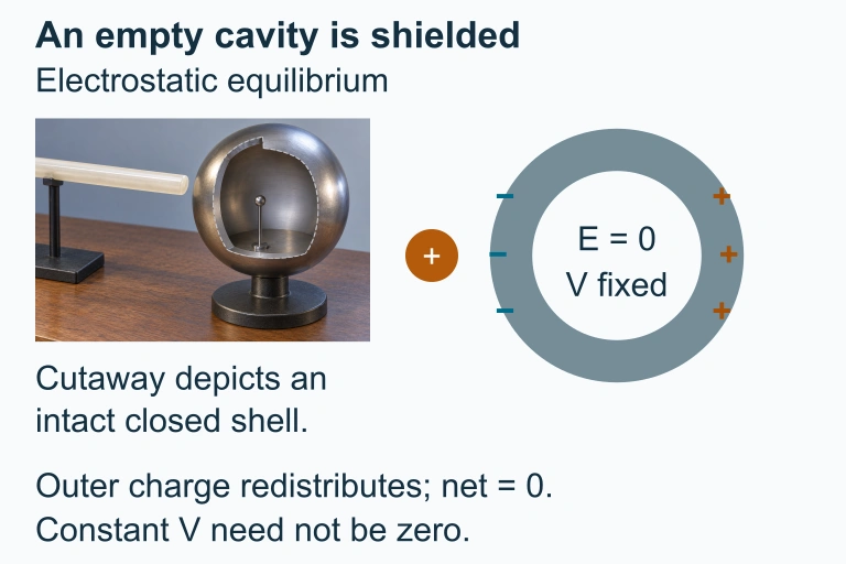External positive charge polarizes closed neutral conductor; empty cavity E=0 and V constant, not necessarily zero. An external charge redistributes charge on a neutral conductor. In electrostatic equilibrium an empty closed cavity has zero electric field and constant potential, which need not be zero.

SECTION 9

Practice Problems

Question 1: CONCEPTUAL

Two positive point charges of equal magnitude are placed a distance d apart. At the exact midpoint between the two charges, the electric field is:

A. Directed from one charge toward the other with a nonzero magnitude
B. Zero, because the fields from the two charges cancel
C. Perpendicular to the line connecting the charges with a nonzero magnitude
D. Directed outward from both charges, doubling the field strength

Show answer (B)

Correct answer: B. At the midpoint, the distance from each charge is d/2, so both fields have the same magnitude E = kQ/(d/2)². However, because both charges are positive, the field from q₁ at the midpoint points away from q₁ (toward q₂), while the field from q₂ points away from q₂ (toward q₁). These two vectors are equal in magnitude and opposite in direction, so they cancel completely, giving E_net = 0. Choice A is wrong because it implies a net field exists, ignoring the opposing directions. Choice C is wrong because there is no mechanism to produce a perpendicular component at this symmetric location. Choice D incorrectly assumes both fields point the same direction, which would be the case if one charge were negative.

Question 2: BASIC CALCULATION

A point charge Q = +6.0 μC creates an electric field. At what distance from the charge is the field magnitude equal to 5.4 × 10⁴ N/C? (Use k = 9.0 × 10⁹ N·m²/C².)

A. 0.10 m
B. 0.50 m
C. 1.0 m
D. 3.0 m

Show answer (C)

Correct answer: C. Starting from E = kQ/r², solve for r: r = √(kQ/E) = √[(9.0 × 10⁹)(6.0 × 10⁻⁶) / (5.4 × 10⁴)] = √[54000 / 54000] = √1 = 1.0 m. Choice A (0.10 m) would give E = 5.4 × 10⁶ N/C, which is 100 times too large. Choice B (0.50 m) yields E = 2.16 × 10⁵ N/C, about 4 times too large. Choice D (3.0 m) yields E = 6.0 × 10³ N/C, which is about 9 times too small. These errors correspond to common mistakes in squaring or taking square roots.

Question 3: INTERMEDIATE

Charge q₁ = +3.0 μC is at the origin and charge q₂ = +3.0 μC is at x = 0.40 m. At what x-coordinate on the axis between the charges is the net electric field zero?

A. x = 0.10 m
B. x = 0.15 m
C. x = 0.20 m
D. x = 0.30 m

Show answer (C)

Correct answer: C. Between two equal positive charges, the zero-field point lies exactly at the midpoint by symmetry. Since q₁ is at x = 0 and q₂ is at x = 0.40 m, the midpoint is x = 0.20 m. At this location, the field from q₁ points in the +x direction (away from q₁) and the field from q₂ points in the −x direction (away from q₂). Equal magnitudes and opposite directions yield E_net = 0. Choice A gives r₁ = 0.10 m and r₂ = 0.30 m, so E₁ would be 9 times larger than E₂ — these cannot cancel. Choice B gives r₁ = 0.15 m and r₂ = 0.25 m, which are unequal, so again E₁ ≠ E₂. Choice D similarly gives asymmetric distances. Only the midpoint produces equal magnitudes for equal charges.

Question 4: APPLIED

5 pts

A student wants to experimentally verify that the electric field between two parallel conducting plates is uniform and determine its magnitude. The student has access to a parallel-plate apparatus with adjustable plate spacing d and a variable DC power supply to set the voltage V across the plates, a small charged pith ball of known charge q and known mass m suspended by an insulating thread, a protractor to measure the angle θ the thread makes with the vertical, and a ruler. (a) Describe a procedure the student should follow to determine the electric field magnitude between the plates for a single trial. (b) What quantities should the student measure and how should they be used to calculate E? (c) Describe how the student could modify the experiment to verify that the field is uniform (same magnitude at different locations between the plates). (d) Identify one significant source of error and explain how it would affect the results. (e) If the student plots E (calculated from the pith ball method) versus V/d, what should the graph look like, and what does the slope represent?

Show answer

Rubric (5 points): Point 1 — Procedure (a): Suspend the charged pith ball between the plates. Turn on the power supply to create a potential difference V across the plates separated by distance d. The electric force on the pith ball causes the thread to deflect from vertical by angle θ. Measure θ with the protractor. In equilibrium, the horizontal electric force equals the horizontal component of tension, and the weight equals the vertical component. Therefore tan θ =

F_E

/ mg = qE / mg, giving E = mg tan θ / q. Point 2 — Measured quantities and calculation (b): Measure the deflection angle θ. Using known values of m, g, and q, calculate E = mg tan θ / q. Alternatively, measure V with a voltmeter and d with a ruler, and compare with E = V/d. Point 3 — Verifying uniformity (c): Reposition the pith ball at several different locations between the plates (varying both the horizontal position between the plates and the vertical height) while keeping V and d constant. If the field is uniform, the deflection angle θ should remain the same at every interior position. A consistent value of E across multiple positions confirms uniformity. Point 4 — Source of error (d): Edge effects (fringing fields): near the edges of the plates, the field lines curve outward and the field is no longer uniform. If the pith ball is too close to the plate edges, the measured field will differ from V/d. This would cause the measured E to be lower than predicted near the edges. Another valid answer: the pith ball's own charge may redistribute charge on the plates, slightly altering the field. Point 5 — Graph analysis (e): The graph of E (from the pith ball measurement) versus V/d should be a straight line through the origin with a slope of 1. This is because the theoretical prediction is E = V/d exactly. A slope of 1 confirms the relationship; deviations from a slope of 1 indicate systematic errors such as charge leakage, fringing, or measurement inaccuracies. Positive bead m=1 mg, q=10 nC at 30°: Tcosθ=mg, Tsinθ=qE, E≈566 N/C.

Positive bead m=1 mg, q=10 nC at 30°: Tcosθ=mg, Tsinθ=qE, E≈566 N/C.

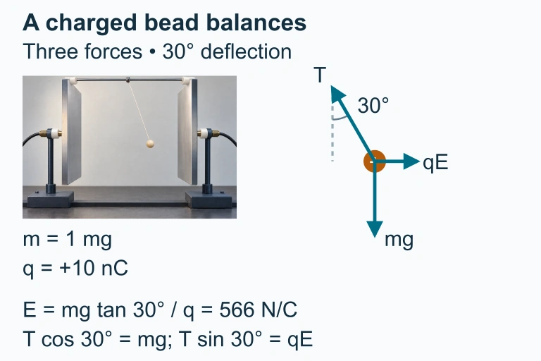At equilibrium the positive bead's electric force balances the horizontal component of tension, while gravity balances its vertical component.

Question 5: CRITICAL THINKING

4 pts

Three charges are arranged at the vertices of an equilateral triangle with side length a = 0.20 m. Charges q₁ = +2.0 μC and q₂ = +2.0 μC occupy the two base vertices (left and right), and charge q₃ = −4.0 μC occupies the top vertex. (a) Determine the direction of the net electric field at the geometric center of the triangle. Justify your answer using a symmetry argument. (b) Calculate the magnitude of the net electric field at the center of the triangle. The distance from each vertex to the centroid of an equilateral triangle with side a is r = a/√3.

Show answer

Rubric (4 points): Point 1 — Symmetry argument for direction (part a): By symmetry, q₁ and q₂ are equal positive charges placed symmetrically about the vertical axis through the center. Each produces an electric field at the center pointing radially away from itself. The horizontal (x) components of E⃗₁ and E⃗₂ are equal in magnitude but opposite in direction, so they cancel. The vertical (y) components of E⃗₁ and E⃗₂ both point upward (away from the base charges toward the top), so they add. The field E⃗₃ from the negative charge q₃ at the top vertex points toward q₃, which is also upward. Therefore, the net electric field at the center points directly upward, toward the top vertex. Point 2 — Distance calculation and individual field magnitudes (part b): The distance from each vertex to the centroid is r = a/√3 = 0.20/√3 ≈ 0.1155 m. The individual field magnitudes are: E₁ = E₂ = kq₁/r² = (9.0 × 10⁹)(2.0 × 10⁻⁶)/(0.1155)² = 1.80 × 10⁴ / 1.333 × 10⁻² ≈ 1.35 × 10⁶ N/C E₃ = k|q₃|/r² = (9.0 × 10⁹)(4.0 × 10⁻⁶)/(0.1155)² = 3.60 × 10⁴ / 1.333 × 10⁻² ≈ 2.70 × 10⁶ N/C Point 3 — Vector component analysis (part b): The centroid lies at height a√3/6 above the base and at horizontal distance a/2 from each base vertex. The line from each base vertex to the centroid makes an angle of 30° above the horizontal, since arctan[(a√3/6)/(a/2)] = arctan(1/√3) = 30°. The electric field from each positive base charge points away from that charge (i.e., from the base vertex toward and beyond the centroid), so each field vector has an upward (y) component of E₁ sin 30° and a horizontal (x) component of E₁ cos 30°. By symmetry, the horizontal components from q₁ and q₂ cancel. The combined upward contribution from q₁ and q₂ is: 2 × E₁ × sin 30° = 2(1.35 × 10⁶)(0.500) ≈ 1.35 × 10⁶ N/C The field from q₃ points entirely upward (toward the negative charge at the top) with magnitude E₃ = 2.70 × 10⁶ N/C. Point 4 — Final magnitude and direction (part b): Summing all upward contributions: E_net = 1.35 × 10⁶ + 2.70 × 10⁶ ≈ 4.05 × 10⁶ N/C The net electric field at the center has magnitude approximately 4.05 × 10⁶ N/C and is directed upward toward the top vertex. This is physically reasonable: the negative charge at the top and the two positive charges at the base all contribute upward field components at the center, reinforcing one another.

SUMMARY

Electric Fields — Summary

Summary

The electric field is a vector quantity defined at every point in space as the force per unit positive test charge: E⃗ = F⃗/q₀. For a point charge, the field magnitude obeys E = kQ/r², decreasing with the inverse square of distance and pointing radially outward for positive Q, inward for negative Q. When multiple charges are present, the superposition principle states that the net field is the vector sum of the individual fields. Electric field lines provide a powerful visual tool: they begin on positive charges, end on negative charges, never cross, and their density encodes the field magnitude.

The parallel-plate configuration produces a uniform electric field (E = V/d) between the plates, making it the standard setup for problems involving charged-particle motion and connections to electric potential. The relationship F⃗ = qE⃗ allows you to predict the force on any charge once the field is known. At a deeper level, the electric field connects to Gauss's law and to equipotential surfaces, forming the conceptual backbone of electrostatics and pointing the way toward the full electromagnetic theory of Maxwell.