Electric Current - AP Physics 2

SECTION 1

Historical Context & Motivation

The study of electricity progressed from curious parlor demonstrations with static charge to the systematic science of electric current over the course of roughly two centuries. Early investigators like Benjamin Franklin recognized that charge could move through conductors, but it was not until the invention of a reliable source of sustained charge flow that quantitative investigation became possible. The development of the voltaic pile in 1800 provided the first continuous source of electrical energy, enabling researchers to study the steady movement of charge through wires and solutions. Each subsequent advance — from Ohm's empirical law to Ampère's precise measurements — deepened our understanding of how and why charge carriers drift in response to an applied electric field, ultimately forming the theoretical backbone of modern circuit analysis.

1745 • The Leyden Jar

Pieter van Musschenbroek invents the Leyden jar, the first device capable of storing significant electric charge, enabling controlled discharge experiments that hinted at the nature of current flow.

1800 • Volta's Pile

Alessandro Volta constructs the first electrochemical battery — stacked discs of zinc, copper, and brine-soaked cardboard — producing the first steady, continuous electric current and launching the age of electrodynamics.

1820 • Ørsted & Ampère

Hans Christian Ørsted demonstrates that a current-carrying wire deflects a magnetic compass needle, and André-Marie Ampère quickly formulates the mathematical relationship between current and magnetic force, defining the unit of current.

1827 • Ohm's Law

Georg Simon Ohm publishes the linear relationship V = IR, establishing that current through a conductor is directly proportional to the applied voltage and inversely proportional to resistance — a cornerstone of circuit analysis.

1897 • Discovery of the Electron

J. J. Thomson identifies the electron as the fundamental charge carrier in metallic conductors, providing a microscopic explanation for macroscopic current and resolving longstanding debates about the nature of electric fluids.

Despite these breakthroughs, the fundamental question at the heart of circuit physics remained: how do we precisely quantify the rate at which charge flows through a conductor, and what microscopic properties of the material govern that rate? Answering this question requires a clear definition of electric current alongside a model connecting macroscopic measurements to the behavior of individual charge carriers. The sections that follow build this framework from the ground up, equipping you to analyze any circuit on the AP Physics 2 exam.

SECTION 2

Core Principles & Definitions

Electric current is fundamentally a measure of how much charge passes a given cross-section of a conductor per unit time. Although it may seem straightforward, several conceptual subtleties distinguish a rigorous understanding from a surface-level one. The following core ideas form the foundation you will apply throughout the study of electric circuits.

Definition of Current

Electric current (I) is defined as the net charge (ΔQ) that passes through a cross-sectional area of a conductor per unit time (Δt). Mathematically, I = ΔQ / Δt, measured in amperes (A), where 1 A = 1 C/s.

Conventional vs. Electron Current

Conventional current is defined as the direction positive charges would move — from higher to lower electric potential. In metallic conductors, the actual charge carriers (electrons) drift in the opposite direction, yet both descriptions yield identical circuit analysis results.

Drift Velocity

Individual electrons in a wire move with a very small average drift velocity (

v_d

), typically on the order of 10⁻⁴ m/s, even though the electric field propagates at nearly the speed of light. The sheer number density of free electrons compensates for this slow drift.

Current Density

Current density (J) is the current per unit cross-sectional area: J = I / A. It is a local quantity that characterizes how concentrated the flow of charge is, and it connects macroscopic current to the microscopic drift model via J = nqv_d.

Conditions for Steady Current

A steady (DC) current requires a closed conducting loop and a sustained potential difference — typically supplied by a battery or power supply. Without a complete circuit, charge cannot flow continuously.

✦

KEY TAKEAWAY

Think of electric current like traffic flow on a highway. The current is analogous to the number of cars passing a toll booth per minute — it does not matter that each individual car moves slowly in bumper-to-bumper traffic. What matters is the collective throughput: a large number of slowly drifting charge carriers (high number density) can produce a substantial current even at extremely low drift velocities. Similarly, the electric signal (like a green traffic light) propagates almost instantly even though the cars themselves creep forward.

SECTION 3

Visual Explanation — Charge Flow in a Conductor

In a metallic conductor, free electrons (cyan circles) drift slowly to the left — opposite to the electric field — while conventional current is drawn in the field direction. Fixed lattice ions (dashed violet circles) remain stationary, providing the periodic potential through which electrons scatter.

The diagram above captures the essential physics of current flow in a metal. When a battery maintains a potential difference across the wire, an internal electric field E develops, directed from the positive terminal toward the negative terminal. This field exerts a force on each free electron (F = qE), accelerating it briefly before it collides with a lattice ion and loses its directed kinetic energy. The net effect of these countless acceleration-and-collision cycles is a small, steady drift velocity superimposed on the electrons' much larger random thermal velocities. Although individual electrons meander chaotically, their average displacement per unit time is directed opposite to E, producing a measurable macroscopic current. Notice that conventional current I points in the same direction as E — from high to low potential — even though the physical carriers drift the other way.

SECTION 4

Mathematical Framework

The mathematical description of electric current bridges two scales: the macroscopic measurement made by an ammeter and the microscopic motion of charge carriers inside the conductor. On the AP Physics 2 exam, you are expected to use the defining equation of current, the drift velocity model, and Ohm's law fluently. Each equation below is accompanied by variable definitions and a physical interpretation.

DEFINITION OF CURRENT

I = ΔQ / Δt

I = electric current (A); ΔQ = net charge passing through a cross-section (C); Δt = elapsed time (s). This equation states that current equals the rate of charge flow. For a steady current, Q = I × t.

DRIFT VELOCITY MODEL

I = nAv_d q

n = number density of free charge carriers (m⁻³); A = cross-sectional area of the conductor (m²); v_d = drift velocity (m/s); q = magnitude of the charge on each carrier (C). This microscopic model connects the collective behavior of charge carriers to the macroscopic current: a larger density, wider wire, or faster drift each increase I.

OHM'S LAW

V = IR

V = potential difference across a resistor (V); I = current through the resistor (A); R = resistance (Ω). Ohm's law is an empirical relation valid for ohmic materials — those whose resistance remains constant over a range of applied voltages. Non-ohmic devices (diodes, LEDs) do not obey this linear relationship.

CURRENT DENSITY

J = I / A = nqv_d

J = current density (A/m²). Current density is useful when analyzing conductors of non-uniform cross-section: at a narrower region, J increases even though I remains constant (conservation of charge), meaning v_d must increase in that segment.

💡

AP Exam Tip

The College Board frequently tests whether students can distinguish between current (a scalar quantity, always positive by convention) and current direction (assigned by circuit convention). When a problem asks for the direction of current, give the conventional direction unless explicitly told otherwise.

SECTION 5

Detailed Breakdown — The Drift Velocity Model

A deeper appreciation of the drift velocity equation I = nAv_dq reveals how each factor independently controls the magnitude of the current. The diagram below illustrates a thought experiment: a cylindrical segment of wire through which charge carriers drift at constant velocity during a time interval Δt.

In a time interval Δt, every charge carrier within the highlighted cylindrical volume (length L = v_d × Δt, cross-sectional area A) passes through the right face. The total charge is the number of carriers in that volume (n × A × L) times the charge per carrier (q), leading directly to I = nAv_d q.

Variable	Symbol & Units	Typical Value (Cu wire)	Effect on I
Number density	n (m⁻³)	8.5 × 10²⁸	I ∝ n — more carriers, more current
Cross-sectional area	A (m²)	≈ 3.3 × 10⁻⁶ (12 AWG)	I ∝ A — wider wire, more current
Drift velocity	$v_d$ (m/s)	≈ 2.3 × 10⁻⁴ (at 10 A)	I ∝ $v_d$ — stronger field, faster drift
Carrier charge	q (C)	1.6 × 10⁻¹⁹	Fixed for electrons in metals

Parameters of the drift velocity model for a standard 12 AWG copper wire

An important consequence of conservation of charge is that the current must be the same at every cross-section of a single, unbranched wire. If the wire narrows, the cross-sectional area A decreases, so the drift velocity v_d must increase proportionally to keep I = nAv_dq constant. This is the electrical analogue of the continuity equation in fluid dynamics: just as water speeds up when a pipe narrows, electrons accelerate through constrictions in a conductor.

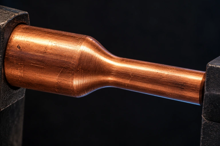Continuous copper neck illustrates smaller cross-section with conserved current. The continuous copper neck is a material illustration. For the separately specified model, the area falls from 2 to 1 mm² while current remains 1 A, so electron drift speed doubles. Conventional current and net electron drift have opposite directions.

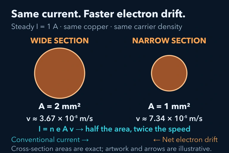I=1 A, n=8.5×10^28 m^-3, areas 2/1 mm² yieldvd 3.67×10^-5/7.34×10^-5 m/s; electron drift opposite conventional current.

SECTION 6

Worked Example — Calculating Drift Velocity

The following problem demonstrates how to combine the definition of current with the drift velocity model to find the speed at which electrons travel through a household wire — a classic AP Physics 2 question type.

Drift Velocity in a 14 AWG Copper Wire

1
Step 1 — Identify Given Values

A 14 AWG copper wire carries a current of I = 5.0 A. The wire has a cross-sectional area A = 2.08 × 10⁻⁶ m². Copper has a free-electron number density of n = 8.5 × 10²⁸ m⁻³, and the electron charge magnitude is q = 1.6 × 10⁻¹⁹ C. We need to find the drift velocity v_d.
2
Step 2 — Select the Appropriate Equation

The drift velocity model relates all the given quantities: I = nAv_dq. Solving for v_d gives: v_d = I / (nAq).
3
Step 3 — Substitute and Compute

v_d = 5.0 / (8.5 × 10²⁸ × 2.08 × 10⁻⁶ × 1.6 × 10⁻¹⁹). First, compute the denominator: 8.5 × 10²⁸ × 2.08 × 10⁻⁶ = 1.768 × 10²³. Then multiply by q: 1.768 × 10²³ × 1.6 × 10⁻¹⁹ = 2.829 × 10⁴. Finally, v_d = 5.0 / 2.829 × 10⁴.

$v_d$ ≈ 1.77 × 10⁻⁴ m/s ≈ 0.18 mm/s
4
Step 4 — Interpret the Result

The drift velocity is astonishingly small — less than 0.2 millimeters per second. This means an individual electron would take over 90 minutes to traverse just one meter of wire. Yet the current begins flowing almost instantaneously when the switch closes because the electric field propagates at nearly the speed of light, setting all electrons in motion simultaneously.
5
Step 5 — Verify Units and Reasonableness

Units check: [A] / ([m⁻³][m²][C]) = [C/s] / [m⁻¹ × C] = [m/s] ✓. The order of magnitude (10⁻⁴ m/s) matches the standard reference value for copper at moderate currents, confirming our answer is physically reasonable.

SECTION 7

DC vs. AC — Comparing Current Types

Electric current comes in two fundamental flavors: direct current (DC), in which the charge carriers flow steadily in one direction, and alternating current (AC), in which they oscillate back and forth periodically. The AP Physics 2 curriculum focuses almost exclusively on DC circuits, but understanding the distinction is essential for connecting classroom physics to the real world and for answering conceptual questions about current behavior.

Property	Direct Current (DC)	Alternating Current (AC)
Direction of flow	Unidirectional — carriers drift in one direction continuously	Reverses periodically, typically sinusoidally at 60 Hz (US) or 50 Hz (EU)
Common sources	Batteries, solar cells, DC power supplies	Wall outlets, generators, transformers
Voltage behavior	Constant (ideally); graph is a horizontal line	Varies sinusoidally between +V_peak and −V_peak
Typical applications	Electronics, sensors, low-voltage circuits	Power transmission, household appliances, industrial motors
AP Physics 2 relevance	Primary focus	Conceptual awareness; not tested quantitatively

Comparison of direct and alternating current characteristics

✦

KEY TAKEAWAY

The distinction between DC and AC is analogous to the difference between a river (steady, one-directional flow) and ocean waves (periodic back-and-forth motion). In both cases, we can define a meaningful flow rate, but the mathematics differs. For AP Physics 2, you will work almost exclusively with the steady-river model (DC), where current is constant and circuit analysis follows directly from Ohm's law and Kirchhoff's rules.

SECTION 8

Connection to Advanced Theory — Non-Ohmic Behavior & Microscopic Models

The simple relationship V = IR works beautifully for resistors and metallic conductors at constant temperature, but the real world is filled with devices whose resistance varies with applied voltage, temperature, or illumination. Understanding where Ohm's law breaks down enriches your conceptual toolkit and connects AP-level circuit physics to the more sophisticated models encountered in college electromagnetism and solid-state physics.

Aspect	AP Physics 2 (Ohmic Model)	Advanced / College Physics
Current–voltage relationship	Linear: I = V/R with constant R	Nonlinear: R depends on V, T, or other parameters
Microscopic model	Drude free-electron model; constant drift velocity per unit field	Band theory; Fermi–Dirac statistics; quantum tunneling in junctions
Temperature dependence	Assumed negligible or qualitatively noted	R(T) modeled with temperature coefficients; superconductivity at T ≈ 0 K
Example devices	Ideal resistors, uniform wires	Diodes, LEDs, thermistors, transistors, photocells
Current density formulation	J = σE (constant conductivity σ)	J = σ(E, T, n)E — conductivity is a function of field, temperature, and carrier concentration

How the current model evolves from AP to advanced physics

On the AP exam, you may encounter qualitative questions about non-ohmic devices — for example, a graph of I vs. V for a light bulb that curves upward because resistance increases as the filament heats. You should be able to interpret such graphs and explain why the slope (1/R) changes. These questions test conceptual reasoning rather than computation and serve as a bridge to the richer physics of semiconductors and quantum materials you will encounter in future courses.

SECTION 9

Practice Problems

Question 1: CONCEPTUAL

When a light switch is flipped, a lamp several meters away turns on almost instantaneously, even though electrons in the wire drift at speeds on the order of 10⁻⁴ m/s. Which of the following best explains this observation?

A. The electrons near the switch travel at the speed of light to the lamp.
B. The electric field established by the battery propagates through the wire at nearly the speed of light, causing all free electrons to begin drifting almost simultaneously.
C. The electrons were already moving at high speed due to thermal energy, and the switch merely redirects that motion.
D. Current only appears to propagate quickly because the lamp's filament has very low thermal inertia.

Show answer (B)

B is correct. The electric field — not the electrons themselves — propagates through the conductor at nearly the speed of light (close to c for most wires). Once the field is established, free electrons throughout the entire circuit begin drifting in response almost simultaneously. Choice A is wrong because individual electrons do not accelerate to the speed of light; they only drift at ~10⁻⁴ m/s. Choice C is wrong because thermal motion is random in direction and does not produce a net current — the switch establishes a directed drift, not a redirection of thermal velocity. Choice D is wrong because even a filament with high thermal inertia would show current flow nearly instantaneously; the speed of light, not the filament's properties, governs signal propagation.

Question 2: BASIC CALCULATION

A steady current of 3.2 A flows through a wire. How much charge passes through a cross-section of the wire in 15 seconds?

A. 0.21 C
B. 4.7 C
C. 48 C
D. 480 C

Show answer (C)

C is correct. Using the definition I = ΔQ / Δt, we rearrange to get ΔQ = I × Δt = 3.2 A × 15 s = 48 C. Choice A (0.21 C) results from dividing current by time instead of multiplying. Choice B (4.7 C) corresponds to dividing 15 by 3.2, which is the wrong operation. Choice D (480 C) results from an arithmetic error, likely misplacing a decimal or multiplying by an extra factor of 10.

Question 3: INTERMEDIATE

A silver wire (n = 5.86 × 10²⁸ m⁻³) has a circular cross-section with diameter 1.0 mm and carries a current of 2.0 A. What is the drift velocity of the free electrons in the wire?

A. 2.7 × 10⁻⁴ m/s
B. 1.1 × 10⁻⁴ m/s
C. 4.3 × 10⁻³ m/s
D. 6.8 × 10⁻⁵ m/s

Show answer (A)

A is correct. First compute the cross-sectional area: r = 0.50 mm = 5.0 × 10⁻⁴ m, so A = πr² = π × (5.0 × 10⁻⁴)² = 7.85 × 10⁻⁷ m². Then use

v_d

= I / (nAq) = 2.0 / (5.86 × 10²⁸ × 7.85 × 10⁻⁷ × 1.6 × 10⁻¹⁹). The denominator evaluates to 5.86 × 10²⁸ × 7.85 × 10⁻⁷ = 4.60 × 10²² ; then 4.60 × 10²² × 1.6 × 10⁻¹⁹ = 7.36 × 10³. So

v_d

= 2.0 / 7.36 × 10³ ≈ 2.7 × 10⁻⁴ m/s. Choice B (1.1 × 10⁻⁴) could result from using the diameter instead of the radius when computing area. Choice C (4.3 × 10⁻³) is off by an order of magnitude, likely from a unit conversion error in the area. Choice D (6.8 × 10⁻⁵) could result from using the area in mm² rather than m².

Question 4: APPLIED

4 pts

An experimental physicist needs to design an experiment to determine whether the relationship between current and voltage for a novel thin-film resistor is ohmic. The available equipment includes a variable DC power supply (0–20 V), a digital ammeter, a digital voltmeter, connecting wires, and the thin-film resistor sample. (a) Describe a procedure the physicist should follow to collect the data needed to determine whether the resistor is ohmic. Include enough detail that another physicist could replicate the experiment. (b) Describe what measurements should be plotted and what feature of the graph would indicate ohmic behavior. (c) Identify one potential source of systematic error in this experiment and explain how it could affect the conclusion. (d) Describe one modification to the procedure that would reduce or eliminate the systematic error identified in part (c).

Show answer

Point-by-point rubric: Part (a) — 1 point: Connect the variable power supply, ammeter (in series), and thin-film resistor in a series loop. Connect the voltmeter in parallel directly across the thin-film resistor's terminals. Set the power supply to a low voltage (e.g., 1.0 V), record both the voltmeter reading (V) and ammeter reading (I). Incrementally increase the supply voltage in equal steps (e.g., 1.0 V intervals) up to 20 V, recording V and I at each setting. Repeat each measurement at least twice for reliability. Part (b) — 1 point: Plot current I (y-axis) vs. voltage V (x-axis). If the resistor is ohmic, the graph will be a straight line passing through the origin. The slope of this line equals 1/R, and its linearity over the entire range confirms constant resistance. Part (c) — 1 point: As current flows through the thin-film resistor, Joule heating raises its temperature. If the resistance is temperature-dependent, higher-voltage data points will reflect a different resistance than lower-voltage points, causing the I–V curve to deviate from linearity even if the material is ohmic at constant temperature. This systematic heating effect could lead to the false conclusion that the resistor is non-ohmic. Part (d) — 1 point: Allow sufficient cooling time between measurements (e.g., 30–60 seconds), or take measurements in quick succession starting from the highest voltage downward and compare with the upward sequence. Alternatively, mount the resistor on a heat sink or immerse it in a temperature-controlled bath to maintain constant temperature throughout the experiment.

Question 5: CRITICAL THINKING

4 pts

A uniform copper wire of length L and cross-sectional area A carries a steady current I. The wire is then replaced with a new copper wire of the same length L but with twice the cross-sectional area (2A), connected to the same battery (assume the battery has negligible internal resistance). (a) Determine the factor by which the current changes when the thicker wire replaces the original. Justify your answer using relevant equations. (b) Determine the factor by which the drift velocity changes. Explain whether your answer is consistent with the drift velocity model I = nAv_d q. (c) A student claims: 'Since the wire is thicker, the electrons have more room, so they slow down, and the current stays the same.' Evaluate this claim.

Show answer

Point-by-point rubric: Part (a) — 1 point: The resistance of a wire is R = ρL/A. Doubling the area halves the resistance: R_new = ρL/(2A) = R/2. By Ohm's law, I = V/R, so the new current is I_new = V/(R/2) = 2V/R = 2I. The current doubles. Part (b) — 1.5 points: From I = nAv_d q, solve for

v_d

v_d

= I/(nAq). With the new wire, I_new = 2I and A_new = 2A, so

v_d

,new = 2I/(n × 2A × q) = I/(nAq) =

v_d

. The drift velocity is unchanged. This is consistent: the current doubled, but the area also doubled, and since

v_d

= I/(nAq), the two factors of 2 cancel. Part (c) — 1.5 points: The student's claim is incorrect. While it is true that a thicker wire gives electrons 'more room' (larger A), the student fails to account for the change in resistance and thus the change in current. The lower resistance of the thicker wire allows more current to flow (I doubles for the same battery voltage). As shown in part (b), the drift velocity actually remains the same — it does not decrease. The current does not stay the same; it increases by a factor of 2. The student's error is treating the current as fixed when in fact it is determined by V/R, which changes when the wire geometry changes.

SUMMARY

Summary — Electric Current

Summary

Electric current (I) is the rate at which charge flows through a conductor, defined by I = ΔQ / Δt and measured in amperes. At the microscopic level, current arises from an enormous number of charge carriers moving at a very small drift velocity, related to macroscopic current by I = nAv_d q. Conventional current flows from high to low potential (the direction positive charges would move), which is opposite to the actual electron drift in metals.

For ohmic materials, Ohm's law (V = IR) provides a linear relationship between voltage and current, enabling straightforward circuit analysis. A steady DC current requires a closed loop and a sustained potential difference. Key exam skills include computing current from charge and time, calculating drift velocity from the microscopic model, and reasoning about how changes in wire geometry or applied voltage affect current. Understanding these principles lays the groundwork for analyzing resistors in series and parallel, Kirchhoff's rules, and power dissipation — the next major topics in the electric circuits unit.