Conservation of Electric Energy - AP Physics 2

SECTION 1

Historical Context & Motivation

The concept of conservation of energy is one of the most powerful unifying principles in all of physics, and its extension to electrical phenomena was neither obvious nor immediate. Before physicists understood that electrical interactions could be described in terms of a potential energy stored in the configuration of charges, the study of electricity was largely phenomenological—scientists catalogued behaviors without a unifying energy framework. The path from Coulomb's force law to a complete energy description of electric systems spanned more than a century of experimental and theoretical work, drawing on advances in mechanics, thermodynamics, and field theory.

1785 • Coulomb's Law Established

Charles-Augustin de Coulomb uses a torsion balance to quantify the force between point charges, demonstrating the inverse-square dependence on distance. This provides the foundation for treating electric interactions as analogous to gravitational ones.

1800 • Volta's Battery

Alessandro Volta invents the voltaic pile, the first device capable of sustaining a continuous electric current. The concept of a potential difference—what we now call voltage—begins to take shape as a measure of energy per unit charge.

1840 • Joule's Heating Experiments

James Prescott Joule demonstrates that electrical energy can be converted into thermal energy, establishing quantitative links between electrical and mechanical forms of energy and reinforcing the conservation principle.

1847 • Helmholtz's Conservation Principle

Hermann von Helmholtz publishes a general statement of energy conservation encompassing mechanical, thermal, and electrical phenomena. This unifies the treatment of electric potential energy within the broader framework of total energy conservation.

1873 • Maxwell's Electromagnetic Theory

James Clerk Maxwell's Treatise on Electricity and Magnetism formalizes the concept of energy stored in electric and magnetic fields. The idea that energy resides not just in charges but in the fields themselves completes the classical picture of electric energy conservation.

The central question that emerged from this history is both elegant and practical: when charges move under the influence of electric forces, how do we systematically track and predict their speeds, positions, and the energy transformations involved? The answer lies in applying the work-energy theorem and the conservation of total mechanical energy to systems of charged particles interacting through the Coulomb force—a conservative force that permits the definition of a well-defined potential energy function.

SECTION 2

Core Principles & Definitions

Conservation of electric energy is not a separate physical law but rather the application of the general conservation of mechanical energy to systems governed by the electrostatic (Coulomb) force. Because the Coulomb force is a conservative force—meaning the work it does on a charge depends only on initial and final positions, not on the path taken—we can define an electric potential energy (U_E) for the system. When no non-conservative forces (such as friction or applied forces) do work, the total mechanical energy—kinetic plus electric potential—remains constant throughout the motion.

Conservative Force

The Coulomb force is path-independent: work done depends only on initial and final positions. This property is essential for defining a potential energy function.

Electric Potential Energy ( $U_E$ )

For two point charges, U_E = kq₁q₂/r. This quantity is positive for like charges (repulsive) and negative for opposite charges (attractive). It represents energy stored in the configuration.

Electric Potential (V)

Electric potential is the potential energy per unit charge: V = U_E/q. It describes the electric landscape that a test charge would experience, measured in volts (J/C).

Energy Conservation Statement

When only conservative (electric) forces act: K_i + U_E,i = K_f + U_E,f. Total mechanical energy is constant.

Potential Difference (ΔV)

The change in electric potential between two points determines the work done per unit charge: W = −qΔV. Charges naturally move from high to low potential energy, converting U_E into K.

✦

KEY TAKEAWAY

Think of electric potential energy as the electrical equivalent of gravitational potential energy. Just as a ball rolls downhill—converting gravitational PE to kinetic energy—a positive charge released near another positive charge "rolls" away through the electric field, converting electric PE to kinetic energy. The total energy remains constant, just as it does for a ball on a frictionless ramp. In engineering applications like particle accelerators, this principle is used to precisely control the final speeds of charged particles by tuning the potential difference through which they are accelerated.

SECTION 3

Visual Explanation

The following diagram illustrates the energy transformation that occurs when a positive charge is released from rest in the vicinity of another fixed positive charge. As the movable charge accelerates away, the electric potential energy of the system decreases while the kinetic energy of the moving charge increases by exactly the same amount, keeping the total mechanical energy constant.

Energy bar charts comparing the initial and final states of a two-charge system. In the initial state (left), the movable charge +q is at rest, so all energy is electric potential energy (yellow bar). In the final state (right), after +q has moved farther away, U_E has decreased and K has increased (cyan bar) by an equal amount. The dashed line shows the constant total energy.

Notice that the total height of the stacked bars remains equal in both panels—this is the visual signature of energy conservation. The yellow bar (U_E) shrinks as the charges separate, while the cyan bar (K) grows by the same amount. If the movable charge were negative instead, it would be attracted toward +Q, the separation would decrease, U_E would become more negative, and K would still increase—consistent with the charge speeding up as it falls into the attractive potential well.

SECTION 4

Mathematical Framework

The mathematical formulation of electric energy conservation begins with the expression for electric potential energy between two point charges, connects to the scalar quantity of electric potential, and culminates in the conservation equation that allows us to solve for unknown velocities, positions, or required potential differences.

ELECTRIC POTENTIAL ENERGY (TWO POINT CHARGES)

U_E = k × q₁ × q₂ / r

Where k = 8.99 × 10⁹ N·m²/C² (Coulomb's constant), q₁ and q₂ are the signed charges (in coulombs), and r is the center-to-center distance between them. The sign of U_E is determined by the signs of the charges: positive for like charges, negative for opposite charges.

ELECTRIC POTENTIAL (VOLTAGE)

V = U_E / q = k × Q / r

The electric potential V at a point in space is the electric potential energy per unit positive test charge. It is a scalar field measured in volts (1 V = 1 J/C). For a point charge Q, V decreases with distance r from the source.

CONSERVATION OF ELECTRIC ENERGY

K_i + U_{E,i} = K_f + U_{E,f}

When only conservative (electric) forces do work, the sum of kinetic energy K and electric potential energy U_E is constant. This is the master equation for solving energy-based problems involving charged particles in electric fields.

WORK-ENERGY FORM (USING POTENTIAL DIFFERENCE)

ΔK = −q ΔV or, for magnitude from rest, ½mv² = |q| × |ΔV|

When a charge q moves through a potential difference ΔV = V_f − V_i, the change in kinetic energy equals −qΔV. For a charge starting from rest, the final speed can be found directly from the magnitude of ΔV. This form is especially useful for uniform electric fields and parallel-plate configurations.

⚠

Sign Convention Reminder

Always include the signs of the charges when computing U_E. A positive U_E indicates a repulsive configuration (like charges), while a negative U_E indicates an attractive configuration (opposite charges). A system with negative U_E is bound—energy must be added to separate the charges to infinity.

SECTION 5

Energy Landscape & Potential Diagrams

One of the most powerful tools for understanding conservation of electric energy is the energy vs. position diagram, which plots the potential energy function U_E(r) as a curve along with a horizontal line representing the total mechanical energy E_total. At any position, the vertical gap between the total energy line and the U_E curve represents the kinetic energy K. Since kinetic energy can never be negative, the charge can only exist in regions where E_total ≥ U_E. The following diagram shows this energy landscape for a repulsive (like-charge) interaction.

For two like charges, the potential energy curve (yellow, U_E ∝ 1/r) rises steeply at small separations. The green dashed line marks the constant total energy. The cyan shaded region between the two curves equals the kinetic energy at each separation. At r_min (the turning point), K = 0 and all energy is potential. As r → ∞, U_E → 0 and K approaches the total energy.

This energy diagram reveals several important physical insights. First, there exists a classical turning point at r_min where the U_E curve intersects the total energy line—the charge momentarily stops and reverses direction at this point, analogous to a ball thrown upward at the top of its trajectory. Second, the kinetic energy at any position is simply the vertical gap between E_total and U_E. Third, as r → ∞, U_E → 0, so the charge's kinetic energy approaches the total mechanical energy—this is the maximum speed the charge can achieve.

Scenario	Sign of $U_E$	Behavior as r decreases	Physical Interpretation
Like charges (+/+ or −/−)	Positive	U_E increases	Repulsive: charges naturally accelerate apart, converting U_E → K
Opposite charges (+/−)	Negative	U_E decreases (more negative)	Attractive: charges naturally accelerate toward each other, converting U_E → K
Charge in uniform E field	U = qEd (linear)	Depends on sign of q and direction of motion relative to E	Analogous to gravity: U_E changes linearly with displacement along field

Summary of electric potential energy behavior in common configurations

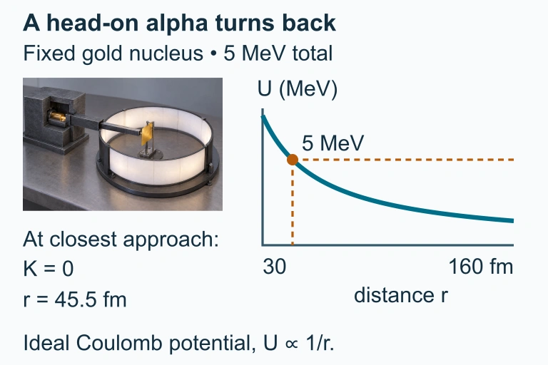Head-on 5 MeV alpha reaches U=5 MeV at r≈45.5 fm; U proportional to 1/r. A head-on 5 MeV alpha particle reaches a closest approach of about 45.5 fm in the ideal fixed-gold Coulomb model, where its kinetic energy becomes zero.

SECTION 6

Worked Example

The following example demonstrates how to apply conservation of electric energy to find the speed of a proton accelerated through a known potential difference—a scenario directly relevant to particle accelerators and cathode ray tubes.

Proton Accelerated Through a Potential Difference

1
Step 1 — Identify Given Values and Goal

A proton (mass m = 1.67 × 10⁻²⁷ kg, charge q = +1.60 × 10⁻¹⁹ C) starts from rest and is accelerated through a potential difference of ΔV = −500 V (it moves from a region of higher potential to lower potential). Find the final speed of the proton.
2
Step 2 — Write the Conservation of Energy Equation

Since only the electric force does work (conservative), we apply: K_i + U_E,i = K_f + U_E,f. Since the proton starts from rest, K_i = 0. Using the relation ΔU_E = qΔV, we rearrange to get: K_f = −qΔV = ½mv².

½mv² = −qΔV
3
Step 3 — Substitute Values

½mv² = −(1.60 × 10⁻¹⁹ C)(−500 V) = 8.00 × 10⁻¹⁷ J. Note that V = J/C, so the units work out to joules. The negative signs cancel because the charge is positive and the potential difference is negative (the proton moves to lower potential), giving a positive kinetic energy as expected.

½mv² = 8.00 × 10⁻¹⁷ J
4
Step 4 — Solve for v

v = √(2 × 8.00 × 10⁻¹⁷ J / 1.67 × 10⁻²⁷ kg) = √(9.58 × 10¹⁰ m²/s²) = 3.10 × 10⁵ m/s. This is about 0.1% of the speed of light, so the non-relativistic treatment is justified.

v ≈ 3.10 × 10⁵ m/s
5
Step 5 — Check Reasonableness

The proton gained kinetic energy equal to 500 eV (since 1 eV = 1.60 × 10⁻¹⁹ J, and the proton has charge +e accelerated through 500 V). This is a typical energy scale for low-energy laboratory experiments. The result is well below relativistic speeds, confirming our classical approach is valid.

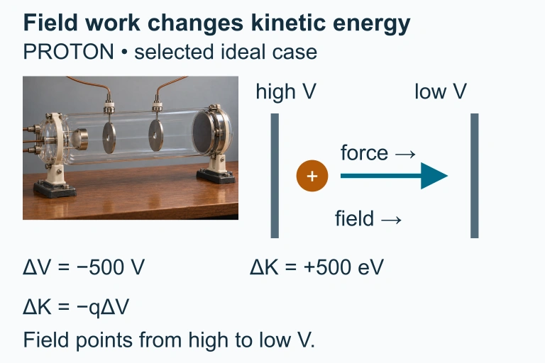Positive proton accelerates from +500 V to 0 V; force follows E; kinetic gain 500 eV. For an ideal particle accelerated through a potential difference, ΔK = −qΔV. The electron case reverses the field direction to accelerate it in the same direction as the proton.

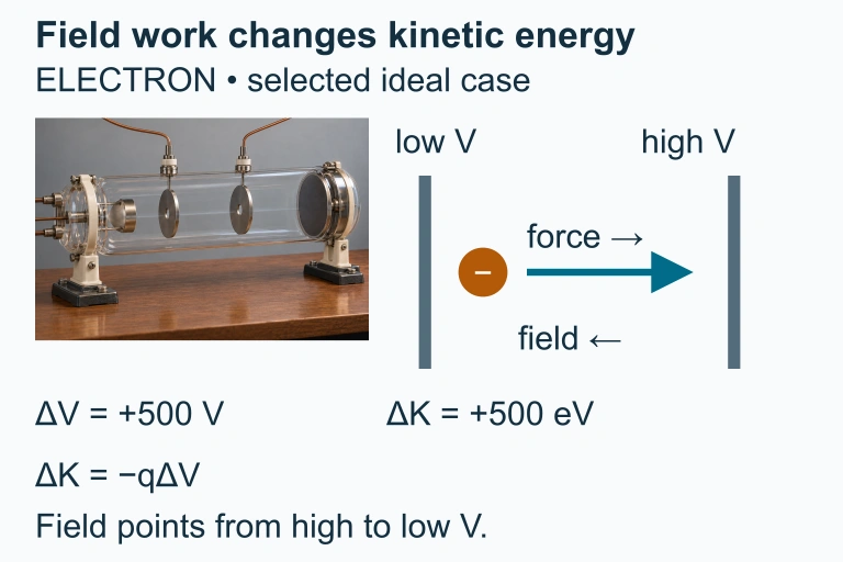Electron gains 500 eV moving from 0 to +500 V, opposite E, with force opposite E. Electron case: reverse field polarity for acceleration to the right.

SECTION 7

Electric vs. Gravitational Energy Conservation

Students often find it helpful to compare conservation of electric energy with the more familiar conservation of gravitational energy, since the mathematical structures are closely analogous. Both arise from inverse-square, conservative forces, and both allow us to replace complicated force-based analysis with elegant scalar energy methods. However, there are crucial differences—most notably that electric charges can be positive or negative, giving rise to both repulsive and attractive potential energies, whereas gravity is always attractive.

Feature	Gravitational Energy	Electric Energy
Force law	F = Gm₁m₂/r²	F = kq₁q₂/r²
Potential energy	U = −Gm₁m₂/r (always negative)	U = kq₁q₂/r (positive or negative)
Nature of interaction	Always attractive	Attractive or repulsive
Source property	Mass (always positive)	Charge (positive or negative)
Relative strength	Extremely weak (G ≈ 6.67 × 10⁻¹¹)	Very strong (k ≈ 8.99 × 10⁹)
Near-surface approximation	U = mgh (linear)	U = qEd (linear, uniform field)
Conservation equation	K_i + U_g,i = K_f + U_g,f	K_i + U_E,i = K_f + U_E,f

Comparison of gravitational and electric energy conservation

✦

KEY TAKEAWAY

The mathematical machinery of energy conservation is identical for gravitational and electric systems—only the source of the potential energy differs. If you can solve a gravitational free-fall problem using mgh, you can solve the analogous electric problem using qΔV. The key new ingredient in electricity is the sign of the charge, which determines whether the particle speeds up moving toward higher or lower potential. This analogy is heavily tested on the AP exam, so building fluency with it is a high-leverage study strategy.

SECTION 8

Connections to Advanced Topics

Conservation of electric energy, as presented in AP Physics 2, is a special case of broader principles that extend into circuit analysis, electromagnetism, and modern physics. Understanding where this framework applies—and where it must be generalized—prepares you for more advanced coursework and provides context for the boundaries of the AP Physics 2 treatment.

AP Physics 2 Treatment	Advanced Extension
Only electrostatic (Coulomb) forces; conservative	Time-varying magnetic fields induce non-conservative electric fields (Faraday's law); potential energy is not always well-defined
Energy stored in charge configurations (U_E = kq₁q₂/r)	Energy stored in the electric field itself: u = ½ε₀E², integrated over all space (field energy density)
Kinetic energy: K = ½mv² (non-relativistic)	For high-speed particles, relativistic energy: E² = (pc)² + (mc²)² replaces classical kinetic energy
Discrete point charges	Continuous charge distributions require integration; capacitor energy U = ½CV² is a key application
Potential difference drives charge motion	In circuits, Kirchhoff's voltage law (ΣΔV = 0 around a loop) is the conservation-of-energy statement applied to current-carrying paths

AP Physics 2 scope vs. advanced generalizations

For AP Physics 2, the most immediately relevant extension is the connection to circuit energy analysis. When you study DC circuits later in the course, you will see that batteries do work on charges by maintaining a potential difference, resistors convert electric energy to thermal energy, and the sum of all energy gains and losses around a closed circuit loop equals zero. This is nothing more than conservation of energy applied to a steady flow of charges, and it is built on the same conceptual foundation established here. Additionally, when charges are accelerated to very high energies—as in particle physics experiments—the electron-volt (eV) becomes the natural unit of energy, defined as the kinetic energy gained by a single elementary charge accelerated through 1 V of potential difference: 1 eV = 1.60 × 10⁻¹⁹ J.

SECTION 9

Practice Problems

Question 1: CONCEPTUAL

A positive charge +q is released from rest at a point midway between two fixed positive charges +Q. Which of the following best describes the subsequent motion and energy transformation of the charge +q?

A. The charge remains stationary because the net electric force is zero at the midpoint.
B. The charge oscillates back and forth, converting kinetic energy to potential energy and back.
C. The charge moves in the direction of any slight displacement, accelerating away from the midpoint as electric potential energy converts to kinetic energy.
D. The charge moves toward one of the fixed charges, gaining potential energy and losing kinetic energy.

Show answer (A)

Choice A is correct. At the exact midpoint, the electric forces from the two equal fixed positive charges cancel. Released exactly from rest in this ideal symmetric system, +q remains there. A small displacement along the line joining the fixed charges produces a restoring force, whereas a transverse displacement produces a force away from the midpoint. Thus the equilibrium is stable axially but unstable transversely; it is not unstable in every direction. Choice B describes a possible perturbed axial motion, not the stated exact release. Choice C incorrectly says any displacement causes runaway motion. Choice D is inconsistent with the stated initial condition and the force direction.

Question 2: BASIC CALCULATION

An electron (mass 9.11 × 10⁻³¹ kg, charge −1.60 × 10⁻¹⁹ C) is accelerated from rest through a potential difference of +200 V. What is the final speed of the electron?

A. 2.65 × 10⁶ m/s
B. 8.39 × 10⁶ m/s
C. 1.67 × 10⁷ m/s
D. 3.10 × 10⁵ m/s

Show answer (B)

The correct answer is B. Using conservation of energy: ½mv² = |q||ΔV|. The electron has charge −e, and moving through ΔV = +200 V means its potential energy decreases (since ΔU = qΔV = (−e)(+200) < 0), so kinetic energy increases. Calculating: ½(9.11 × 10⁻³¹)v² = (1.60 × 10⁻¹⁹)(200) = 3.20 × 10⁻¹⁷ J. Solving: v = √(2 × 3.20 × 10⁻¹⁷ / 9.11 × 10⁻³¹) = √(7.03 × 10¹³) ≈ 8.39 × 10⁶ m/s. Choice A is off by roughly a factor of √10, suggesting an arithmetic error in the power of ten. Choice C doubles the correct answer, possibly from omitting the factor of ½ in the kinetic energy formula. Choice D is the speed a proton (not an electron) would achieve through 500 V, confusing the particle mass.

Question 3: INTERMEDIATE

Two point charges, q₁ = +3.0 μC and q₂ = −5.0 μC, are initially separated by 0.40 m. If they are released from rest, what is the speed of each charge when their separation has decreased to 0.20 m? Assume q₁ has mass m₁ = 2.0 × 10⁻³ kg and q₂ has mass m₂ = 4.0 × 10⁻³ kg.

A. v₁ = 5.8 m/s, v₂ = 2.9 m/s
B. v₁ = 4.1 m/s, v₂ = 4.1 m/s
C. v₁ = 2.9 m/s, v₂ = 5.8 m/s
D. v₁ ≈ 15.0 m/s, v₂ ≈ 7.5 m/s

Show answer (D)

The correct answer is D. This problem requires both conservation of energy and conservation of momentum. Since the charges start from rest, the total momentum is zero, so m₁v₁ = m₂v₂. With m₁ = 2.0 × 10⁻³ kg and m₂ = 4.0 × 10⁻³ kg, this gives v₁ = 2v₂. The change in electric potential energy is ΔU_E = kq₁q₂(1/r_f − 1/r_i) = (8.99 × 10⁹)(3.0 × 10⁻⁶)(−5.0 × 10⁻⁶)(1/0.20 − 1/0.40). First, kq₁q₂ = (8.99 × 10⁹)(−1.5 × 10⁻¹¹) = −0.13485 J·m. Then (1/0.20 − 1/0.40) = (5.0 − 2.5) = 2.5 m⁻¹. So ΔU = (−0.13485)(2.5) = −0.337 J. Since the charges attract (opposite signs), potential energy decreases as they move closer, and kinetic energy increases by 0.337 J. Using ½m₁v₁² + ½m₂v₂² = 0.337 J with v₁ = 2v₂: ½(2.0 × 10⁻³)(2v₂)² + ½(4.0 × 10⁻³)(v₂²) = 0.004v₂² + 0.002v₂² = 0.006v₂² = 0.337. So v₂² = 56.17, giving v₂ ≈ 7.5 m/s and v₁ = 2v₂ ≈ 15.0 m/s. Choice A is incorrect because those speeds are too low and correspond to a much smaller energy change. Choice B is incorrect because equal speeds violate conservation of momentum when the masses differ. Choice C is incorrect because the lighter charge must move faster, not slower. Choice D is correct with the properly calculated speeds.

Question 4: APPLIED

4 pts

A research team wants to test conservation of mechanical energy for a small, point-like bead of known mass m and positive charge q moving on a horizontal frictionless track between two vertical parallel plates. The plates produce a uniform horizontal field E in the +x direction; their separation is d and their positive voltage difference is V. The start and end points lie away from edge fields. (a) Describe a procedure, including quantities to measure and vary. (b) Explain how to analyze the data. (c) Identify one systematic error and its effect. (d) Explain how to adapt the analysis if the field is non-uniform.

Show answer

Point 1 — Procedure (1 pt): Measure m, q, plate separation d, voltage difference V, horizontal displacement Δx along +x, and the initial and final speeds vi and vf using photogates or video. Repeat for several V values while keeping geometry and release conditions fixed. The track is horizontal and the bead model has no rotational kinetic energy. Point 2 — Analysis (1 pt): Calculate ΔK = ½m(vf² − vi²). For motion along E, the signed potential change is ΔV = −EΔx = −(V/d)Δx, so ΔUE = qΔV and ΔK = −ΔUE = q(V/d)Δx if electric work is the only energy transfer to motion. Plot ΔK versus −qΔV and compare the fitted slope with 1 and intercept with 0, accounting for uncertainties. V is the positive plate-voltage difference; ΔV is the signed change from the bead's start to end point. A mismatch signals neglected effects or measurement uncertainty, not failure of total energy conservation. Point 3 — Systematic error (1 pt): Drag or track friction transfers energy to thermal forms, making ΔK smaller than −qΔV. The bead-plus-field mechanical energy then decreases, but energy is conserved in the larger system including the surroundings. Point 4 — Non-uniform field (1 pt): Use a known or independently calibrated potential distribution to determine the signed endpoint ΔV, or integrate ΔV = −∫E·dl along the path. The relation ΔK = −qΔV still applies under the same mechanical assumptions. An ordinary voltmeter is not a direct probe of the potential at an unconnected point in empty space.

Question 5: CRITICAL THINKING

4 pts

Three identical positive point charges, each of magnitude +Q, are initially held at the vertices of an equilateral triangle with side length L. (a) Derive an expression for the total electric potential energy of the three-charge system in terms of k, Q, and L. (b) If all three charges are released simultaneously, determine the speed of each charge when they are very far apart from one another. Express your answer in terms of k, Q, L, and the mass m of each charge. (c) Explain why conservation of momentum guarantees that all three charges must have the same final speed. (d) If one of the three charges were instead −Q, describe qualitatively how the motion and energy transformation would differ.

Show answer

Point 1 — Total Potential Energy (1 pt): The system has three pairs of interactions: (1,2), (1,3), and (2,3). Each pair contributes U = kQ²/L. Since all three pairs are identical: U_total = 3kQ²/L. Point 2 — Final Speed Derivation (1 pt): When the charges are infinitely far apart, U_f = 0. By conservation of energy: 0 + 3kQ²/L = 3(½mv²) + 0. Solving: 3kQ²/L = (3/2)mv² → v = √(2kQ²/(mL)). Point 3 — Momentum Argument (1 pt): The initial total momentum is zero (all charges at rest). By conservation of momentum, the total momentum must remain zero at all times. Since all three charges have identical mass and charge and start in a symmetric configuration (equilateral triangle), the three-fold rotational symmetry is preserved throughout the motion. Each charge moves radially outward along its respective line of symmetry with the same speed. If any one charge had a different speed, the vector sum of momenta would not be zero, violating conservation of momentum. Point 4 — Qualitative Analysis with −Q (1 pt): Replacing one charge with −Q breaks the symmetry. The initial potential energy would be U = kQ²/L + 2k(Q)(−Q)/L = kQ²/L − 2kQ²/L = −kQ²/L (negative, indicating a bound system). The two positive charges would repel each other but both would be attracted toward the negative charge. The negative charge would not simply fly away; instead, the system's behavior becomes complex. Because U_total < 0, there is not enough energy for all three charges to escape to infinity—the system is energetically bound, and at least two of the charges must remain in a bound configuration.

SUMMARY

Summary & Key Concepts

Summary

Conservation of electric energy applies the general principle of conservation of mechanical energy to systems of charges interacting through the conservative Coulomb force. The fundamental equation is $K_i$ + $U_{E,i}$ = $K_f$ + $U_{E,f}$ , where the electric potential energy for two point charges is U_E = kq₁q₂/r. The sign of U_E is determined by the signs of the charges: positive for repulsive (like-charge) configurations and negative for attractive (opposite-charge) configurations.

When a charge moves through a potential difference ΔV, its change in kinetic energy is ΔK = −qΔV, which provides a powerful shortcut for uniform-field and parallel-plate problems. The electron-volt (eV) is a convenient energy unit equal to 1.60 × 10⁻¹⁹ J. The mathematical structure is directly analogous to gravitational energy conservation, with electric potential energy playing the role of gravitational potential energy. Master the signs, practice with energy bar charts, and remember: when only electric forces act, the total mechanical energy of the system never changes.