

SECTION 1
Historical Context & Motivation
The study of oscillatory motion dates back centuries, rooted in humanity's earliest encounters with pendulums, vibrating strings, and celestial cycles. The formal mathematical treatment of simple harmonic motion (SHM) grew from efforts to describe how objects move back and forth around a stable equilibrium position. What makes SHM so central to physics is that it serves as the universal model for any system experiencing a restoring force proportional to displacement — from atoms in a crystal lattice to the oscillations of a guitar string. Understanding how to represent and analyze SHM graphically and mathematically unlocks insights across mechanics, waves, sound, and even quantum physics.
1583 • Galileo and the Pendulum
1656 • Huygens' Pendulum Clock
1678 • Hooke's Law
1736 • Euler's Sinusoidal Functions
1822 • Fourier Analysis
These historical developments converge on a central question: How do we precisely describe the position, velocity, acceleration, and energy of an oscillator at every instant? The answer lies in sinusoidal representations and the phase relationships among kinematic quantities — tools that remain essential in the AP Physics 1 curriculum and well beyond.
SECTION 2
Core Principles & Definitions
Before diving into graphs and equations, it is essential to establish the foundational vocabulary and physical ideas that govern SHM. Every oscillating system that qualifies as simple harmonic exhibits a linear restoring force directed toward equilibrium and proportional to the displacement from that equilibrium. This single condition dictates sinusoidal motion, fixed-period oscillations, and predictable energy exchange between kinetic and potential forms.
Amplitude (A)
Period (T) & Frequency (f)
Angular Frequency (ω)
Phase Constant (φ₀)
Restoring Force & Equilibrium
KEY TAKEAWAY
SECTION 3
Visual Explanation — x(t), v(t), and a(t) Graphs
The most powerful way to understand SHM is to examine how position, velocity, and acceleration evolve over time on stacked sinusoidal graphs. These three curves have identical shapes — all sinusoidal with the same period — but they are phase-shifted relative to one another. Velocity leads position by a quarter cycle (π/2 radians), and acceleration leads velocity by another quarter cycle. Equivalently, acceleration is exactly half a cycle (π radians) out of phase with position, which is the graphical signature of the restoring force always opposing displacement.
Several crucial relationships emerge from these graphs. At the moment the position reaches its maximum displacement (x = +A), the velocity is zero and the acceleration has its maximum magnitude in the negative direction. Conversely, when the object passes through equilibrium (x = 0), the velocity reaches its maximum magnitude while the acceleration is zero. These relationships are not coincidental — they are direct consequences of Newton's second law applied to a restoring force: the acceleration must always point opposite to the displacement.
AP Exam Tip
 One coordinate of a peg in uniform circular motion varies sinusoidally. The spring cart provides a second oscillator model in which acceleration points toward equilibrium.
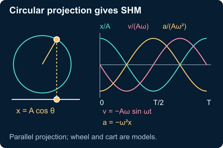 One coordinate of a peg in uniform circular motion varies sinusoidally. The spring cart provides a second oscillator model in which acceleration points toward equilibrium.
SECTION 4
Mathematical Framework
The sinusoidal functions that describe SHM are not arbitrary — they are the unique solutions to the condition that acceleration is proportional to, and opposite in direction from, displacement. For an object oscillating along the x-axis with amplitude A, angular frequency ω, and initial phase φ₀, the three kinematic equations of SHM follow directly from one another through differentiation.
POSITION
A = amplitude (m), ω = angular frequency (rad/s), t = time (s), φ₀ = initial phase (rad). The cosine form is conventional when the object starts at maximum displacement.
VELOCITY
The maximum speed is vmax = Aω, which occurs as the object passes through equilibrium. The negative sign ensures that velocity is the time derivative of position.
ACCELERATION
The maximum acceleration magnitude is amax = Aω². Note that a = −ω²x, confirming that acceleration is always proportional to and opposite in sign from displacement.
ANGULAR FREQUENCY RELATIONS
For a mass-spring system: ω = √(k/m). For a simple pendulum (small angle): ω = √(g/L). These connect the abstract angular frequency to physical system parameters.
A critical insight is the relationship a(t) = −ω²x(t). This equation encapsulates the defining property of SHM: the acceleration is always proportional to the displacement with a negative proportionality constant. When you encounter a system where this relationship holds, you can immediately conclude the motion is simple harmonic and identify ω² as the coefficient. On the AP exam, being able to recognize this form — whether given as an equation, a graph, or a verbal description — is essential for earning full credit on both multiple-choice and free-response questions.
Phase Constant Conventions
SECTION 5
Energy in SHM — KE, PE, and Total Energy
Energy analysis provides a complementary perspective on SHM that the AP exam tests heavily. In an ideal (frictionless) oscillator, total mechanical energy is conserved and continuously converts between kinetic energy (KE) and potential energy (PE). At the equilibrium position, all energy is kinetic; at the turning points (x = ±A), all energy is potential. Importantly, both KE and PE vary sinusoidally with twice the frequency of the displacement — the energy completes a full cycle in half the period because PE peaks at both +A and −A.
ENERGY EQUATIONS
At any displacement x, PE = ½kx² and KE = ½k(A² − x²). The total energy E = ½kA² depends on amplitude squared, so doubling the amplitude quadruples the energy.
The energy-position diagram is an especially powerful tool because it allows you to determine the speed at any position without knowing the time. Given E = ½kA² and PE = ½kx², the kinetic energy at any x is KE = ½k(A² − x²), so the speed at position x is v = ω√(A² − x²). At x = 0, this simplifies to vmax = Aω. At x = ±A, v = 0 as expected. Many AP free-response questions ask you to relate speed and position using this energy approach, which avoids the need to solve for time explicitly.
SECTION 6
Worked Example
Mass-Spring Oscillator: Full Kinematic & Energy Analysis
- 1
Step 1 — Identify Given Values
A 0.50 kg block is attached to a horizontal spring (k = 200 N/m) on a frictionless surface. The block is pulled 0.10 m from equilibrium and released from rest. Find the period, maximum speed, maximum acceleration, and the speed when the block is 0.060 m from equilibrium. - 2
Step 2 — Calculate Angular Frequency and Period
ω = √(k/m) = √(200/0.50) = √400 = 20 rad/s. The period is T = 2π/ω = 2π/20 = 0.314 s.T ≈ 0.314 s, ω = 20 rad/s - 3
Step 3 — Find Maximum Speed
The maximum speed occurs at equilibrium: vmax = Aω = (0.10 m)(20 rad/s) = 2.0 m/s. Alternatively, using energy: ½mv² = ½kA² gives v = A√(k/m) = 0.10 × 20 = 2.0 m/s.v_max = 2.0 m/s - 4
Step 4 — Find Maximum Acceleration
The maximum acceleration occurs at maximum displacement: amax = Aω² = (0.10 m)(20 rad/s)² = (0.10)(400) = 40 m/s². This can also be found from Newton's second law: amax = kA/m = (200)(0.10)/0.50 = 40 m/s².a_max = 40 m/s² - 5
Step 5 — Find Speed at x = 0.060 m
Using the energy-derived velocity equation: v = ω√(A² − x²) = 20 × √(0.10² − 0.060²) = 20 × √(0.0100 − 0.0036) = 20 × √(0.0064) = 20 × 0.080 = 1.6 m/s. The block retains significant speed because it is still relatively close to equilibrium.v = 1.6 m/s at x = 0.060 m
Dimensional Check
SECTION 7
Comparing Representations of SHM
SHM can be described through multiple representations — verbal descriptions, equations, graphs, energy bar charts, and motion diagrams. The AP Physics 1 exam rewards students who can fluently translate between these representations. Each has strengths and limitations, and the table below summarizes when each is most useful.
| Representation | Strengths | Limitations |
|---|---|---|
| Sinusoidal Equations | Provide exact values of x, v, or a at any time; reveal phase relationships analytically; allow algebraic derivations of energy and velocity at any position. | Require knowledge of ω, A, and φ₀; abstract for students who think visually; don't immediately convey qualitative behavior. |
| x(t), v(t), a(t) Graphs | Show phase shifts visually; make it easy to identify maxima, zeros, and turning points; slopes connect kinematics (slope of x is v, slope of v is a). | Hard to extract precise numerical values without a scale; require careful axis labeling to avoid sign errors. |
| Energy vs. Position Graph | Directly shows KE, PE, and total E at any position; illustrates energy conservation; can determine speed at any x without time. | Contains no time information; cannot tell how fast the object reaches a given position; does not show direction of motion. |
| Energy Bar Charts | Excellent for qualitative comparisons at different positions; clearly show energy transfer from KE to PE and back. | Not suitable for precise calculations; only show discrete snapshots, not continuous motion. |
| Motion Diagrams | Show how position and velocity change over equal time intervals; make the 'speeding up near equilibrium, slowing near turning points' pattern intuitive. | Difficult to read for more than one full cycle; do not encode acceleration explicitly. |
Comparison of SHM representations used on the AP Physics 1 exam
KEY TAKEAWAY
SECTION 8
Connection to Advanced Theory
Simple harmonic motion is the idealized case — the first term in a broader description of oscillatory systems. Understanding how the AP Physics 1 treatment connects to more advanced concepts helps you appreciate both the power and the boundaries of the SHM model.
| AP Physics 1 (SHM) | Advanced Extension |
|---|---|
| No friction or damping; amplitude stays constant forever. | Damped oscillations: amplitude decays exponentially due to viscous or friction forces (AP Physics C and beyond). |
| Restoring force is exactly proportional to displacement (F = −kx). | Anharmonic oscillations: for large displacements, restoring forces become nonlinear (e.g., pendulum at large angles), and period depends on amplitude. |
| System oscillates at its natural frequency only. | Driven and resonant oscillations: an external periodic force can drive the system and, at resonance, produce dramatic amplitude growth. |
| Single-particle oscillation; no wave propagation. | Coupled oscillators and mechanical waves: SHM of individual particles underpins traveling and standing waves. |
| Classical description using position and momentum. | Quantum harmonic oscillator: energy is quantized into discrete levels = (n + ½)ℏω, the foundation of quantum field theory. |
From AP Physics 1 SHM to more advanced oscillatory theory
The key forward-looking idea for AP students is this: when you study mechanical waves later in the course, you will see that each small element of the medium undergoes SHM. The wave equation itself is built by coupling many simple harmonic oscillators together, so the sinusoidal mathematics you have learned here — amplitude, frequency, phase — will reappear as the fundamental language of wave phenomena, from sound to light.
SECTION 9
Practice Problems
Question 1: CONCEPTUAL
- A. The velocity is zero and the acceleration is at its maximum magnitude.
- B. The velocity is at its maximum magnitude and the acceleration is zero.
- C. Both the velocity and the acceleration are at their maximum magnitudes.
- D. Both the velocity and the acceleration are zero.
Show answer (B)
Question 2: BASIC CALCULATION
- A. 0.80 m/s
- B. 1.6 m/s
- C. 2.0 m/s
- D. 3.2 m/s
Show answer (B)
Question 3: INTERMEDIATE
- A. A/2
- B. A√3/2
- C. A/4
- D. A/√2
Show answer (B)
Question 4: APPLIED
5 ptsShow answer
Question 5: CRITICAL THINKING
4 ptsShow answer
SUMMARY
Summary
Summary
Simple harmonic motion describes any oscillation where the restoring force is proportional to displacement (F = −kx), producing sinusoidal position, velocity, and acceleration functions. The motion is fully characterized by three parameters: amplitude A (maximum displacement), angular frequency ω = 2π/T (which depends on system properties, not amplitude), and phase constant φ₀ (set by initial conditions). The position x(t) = A cos(ωt + φ₀), velocity v(t) = −Aω sin(ωt + φ₀), and acceleration a(t) = −ω²x(t) are related by quarter-cycle phase shifts — velocity leads position by π/2, and acceleration is π out of phase with position.
Energy in SHM oscillates between kinetic energy (½mv², maximum at equilibrium) and potential energy (½kx², maximum at turning points), with total mechanical energy E = ½kA² conserved throughout. The energy-position parabolas allow determination of speed at any displacement via v = ω√(A² − x²). Mastery of SHM requires fluency in translating between equations, graphs, energy diagrams, and verbal descriptions — a skill the AP exam tests extensively across both MCQ and FRQ formats.