

SECTION 1
Historical Context & Motivation
The concept of thermal pollution emerged alongside the rapid industrialization of the nineteenth and twentieth centuries. As coal-fired and later nuclear power plants proliferated, engineers recognized that the massive volumes of cooling water discharged back into rivers, lakes, and coastal zones carried significantly elevated temperatures. Early environmental observers noted fish kills and shifts in aquatic community composition downstream of industrial outfalls, but the problem received little regulatory attention until the mid-twentieth century. The recognition that heat itself could function as a pollutant—degrading dissolved oxygen, altering metabolic rates, and reshaping species assemblages—represented an important conceptual shift in environmental science.
1830s–1880s • Industrial Revolution Expansion
1962 • Silent Spring Sparks Awareness
1972 • Clean Water Act (CWA)
1990s–Present • Climate Change Synergies
The central question thermal pollution poses is straightforward yet ecologically profound: How does an anthropogenic change in water temperature cascade through physical, chemical, and biological processes to alter an entire aquatic ecosystem? Answering this question requires integrating thermodynamics, aquatic chemistry, and population ecology—precisely the interdisciplinary perspective that AP Environmental Science cultivates.
SECTION 2
Core Principles & Definitions
Thermal pollution occurs when human activity alters the temperature of a natural water body enough to produce adverse ecological or chemical effects. Although most commonly associated with heated effluent, the phenomenon also encompasses artificially cooled discharges—such as those from liquefied natural gas facilities—that can shock cold-sensitive organisms. Understanding thermal pollution requires familiarity with several interconnected principles governing how heat interacts with aquatic systems.
Dissolved Oxygen & Temperature
Metabolic Rate Acceleration
Thermal Shock
Thermal Plume
Biological Oxygen Demand (BOD)
SECTION 3
Visual Explanation — The Thermal Plume
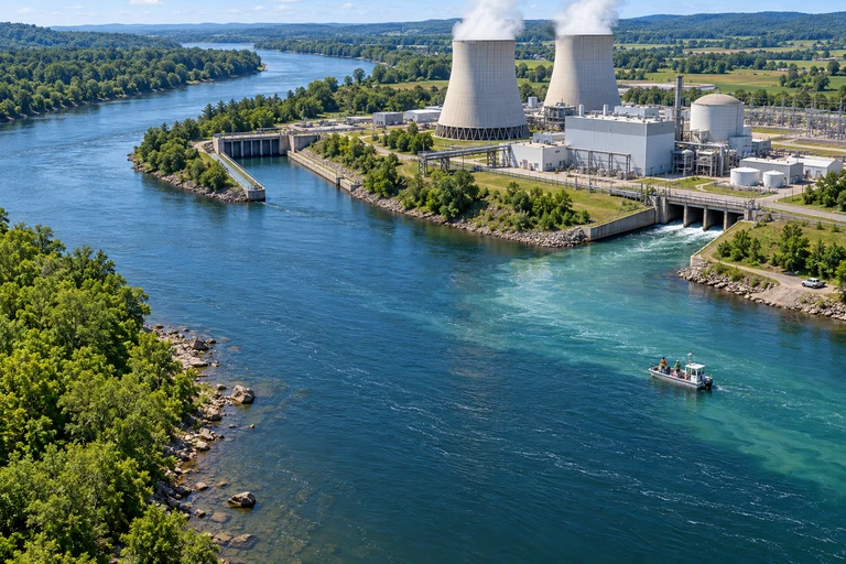
The thermal plume is not merely a temperature gradient—it is an ecological filter. Species unable to tolerate elevated temperatures are excluded from Zone A, creating an artificially simplified community with lower biodiversity. Meanwhile, organisms adapted to warmer conditions (often invasive or pollution-tolerant species) may colonize the plume, fundamentally altering trophic dynamics. The spatial extent of the plume depends on the volume and temperature of the discharge, the flow rate and mixing capacity of the receiving water body, and prevailing meteorological conditions.
 Suppose 50 m³/s is diverted from a 200 m³/s river at 15°C and returned 10°C warmer. Under the stated steady mixing balance, the recombined 200 m³/s flow reaches 17.5°C. Oxygen conditions also depend on oxygen demand, reaeration and other site conditions.
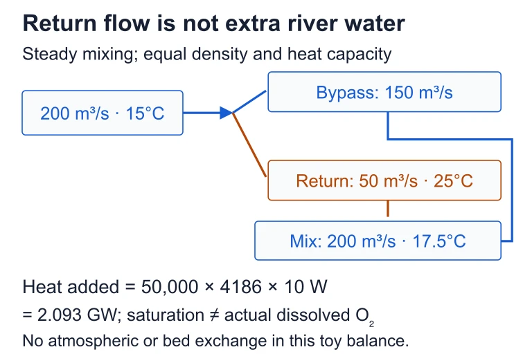 Suppose 50 m³/s is diverted from a 200 m³/s river at 15°C and returned 10°C warmer. Under the stated steady mixing balance, the recombined 200 m³/s flow reaches 17.5°C. Oxygen conditions also depend on oxygen demand, reaeration and other site conditions.
SECTION 4
Mathematical Framework
Quantifying thermal pollution involves calculating the rate of heat transfer to a water body and predicting the resulting temperature change. The fundamental relationship links the mass flow rate of cooling water, the specific heat capacity of water, and the temperature differential between the intake and discharge.
HEAT DISCHARGED
Where Q = rate of heat energy discharged (J/s or watts), ṁ = mass flow rate of cooling water (kg/s), c = specific heat capacity of water (4,186 J/(kg·°C)), ΔT = temperature difference between discharge and intake (°C).
TEMPERATURE RISE IN RECEIVING WATER
This equation estimates the temperature increase in the receiving water body after complete mixing. ṁ_river is the mass flow rate of the river (kg/s). Higher river flow means greater dilution capacity and a smaller temperature rise.
DISSOLVED OXYGEN SATURATION (SIMPLIFIED)
An empirical approximation where DO_sat is the saturation concentration of dissolved oxygen (mg/L) and T is water temperature (°C) at 1 atm. This illustrates the inverse relationship between temperature and oxygen solubility.
SECTION 5
Sources, Effects, and Ecological Consequences
Among all sources, thermoelectric power plants are the single largest contributors to thermal pollution in the United States, collectively withdrawing roughly 40% of all freshwater for cooling purposes. Nuclear plants tend to produce more waste heat per unit of electricity than fossil-fuel plants because their thermodynamic efficiency is lower (≈ 33% vs. ≈ 40%), meaning a greater proportion of fuel energy must be rejected as heat. Urban stormwater runoff is an often-overlooked source: paved surfaces absorb solar radiation, and rainfall flowing over asphalt can be 10–15 °C warmer than ambient stream temperature. Deforestation of riparian buffer zones removes canopy shading, exposing streams to direct solar heating and raising baseline temperatures.
| Source | Typical ΔT (°C) | Primary Receiving Water |
|---|---|---|
| Coal-fired power plant | +5 to +10 | Rivers, lakes, estuaries |
| Nuclear power plant | +8 to +15 | Rivers, coastal ocean |
| Urban stormwater runoff | +10 to +15 | Urban streams, wetlands |
| Riparian deforestation | +2 to +6 | Headwater streams |
| Industrial cooling (steel, chemical) | +6 to +12 | Rivers, estuaries |
Representative temperature increases by thermal pollution source.
SECTION 6
Worked Example — Calculating Thermal Discharge and DO Impact
A coal-fired power plant draws cooling water from a river at 15 °C and discharges it at 25 °C. The plant uses 50 m³/s of cooling water. The river's flow rate is 200 m³/s. Estimate the heat energy discharged per second and the temperature rise in the river after complete mixing. Then evaluate the change in dissolved oxygen saturation.
Worked example
- 1
Step 1 — Identify Given Values
Intake temperature T_in = 15 °C; Discharge temperature T_out = 25 °C; ΔT = 25 − 15 = 10 °C. Cooling water flow rate = 50 m³/s. Density of water ≈ 1,000 kg/m³, so ṁ = 50,000 kg/s. Specific heat c = 4,186 J/(kg·°C). River flow rate = 200 m³/s → ṁ_river = 200,000 kg/s. - 2
Step 2 — Calculate Heat Discharged
Q = ṁ × c × ΔT = 50,000 kg/s × 4,186 J/(kg·°C) × 10 °CQ = 2.093 × 10⁹ J/s ≈ 2.09 GW of waste heat - 3
Step 3 — Calculate River Temperature Rise
After complete mixing, ΔT_river = Q / (ṁ_river × c) = 2.093 × 10⁹ / (200,000 × 4,186)ΔT_river ≈ 2.5 °C → River rises from 15 °C to 17.5 °C - 4
Step 4 — Evaluate DO Change
Using DO_sat ≈ 14.6 − 0.39T + 0.0072T²: At 15 °C → DO ≈ 14.6 − 5.85 + 1.62 = 10.37 mg/L. At 17.5 °C → DO ≈ 14.6 − 6.825 + 2.205 = 9.98 mg/L.DO saturation decreases by ≈ 0.39 mg/L (a 3.8% decline) - 5
Step 5 — Ecological Interpretation
A 2.5 °C temperature rise with a corresponding DO decline of ~0.4 mg/L may seem small, but for cold-water species like trout (which require DO > 7 mg/L and temperatures < 20 °C), even this shift pushes conditions closer to critical thresholds, particularly during summer when ambient temperatures are already elevated.
SECTION 7
Mitigation Strategies — Strengths & Limitations
A variety of engineering and ecological strategies exist to mitigate thermal pollution. Each involves trade-offs between cost, water consumption, land use, and ecological effectiveness. Understanding these trade-offs is essential both for the AP exam and for real-world environmental management.
| Strategy | Strengths | Limitations |
|---|---|---|
| Cooling towers | Dramatically reduce thermal discharge; can lower effluent to near-ambient temperatures | High construction cost; evaporative losses consume water and may create local fog and salt drift |
| Cooling ponds / reservoirs | Low-tech; natural heat dissipation through evaporation and radiation | Require large land area; still lose water to evaporation; may develop algal blooms |
| Cogeneration (CHP) | Captures waste heat for industrial/domestic heating; overall efficiency >80% | Requires proximity to heat consumers; complex infrastructure; seasonal heat demand variation |
| Riparian buffer restoration | Provides shading, reduces solar heating, stabilizes banks, adds habitat | Addresses only solar-driven heating; decades to mature; insufficient for large industrial discharges |
| Closed-loop cooling systems | Minimal thermal discharge; water is recirculated through cooling towers | Most expensive option; higher energy parasitic load on the plant; still has evaporative loss |
Comparison of thermal pollution mitigation approaches.
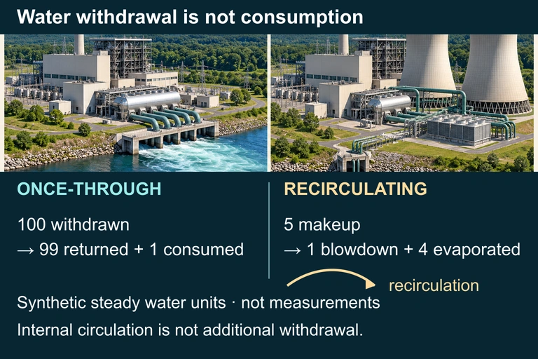 In the synthetic steady comparison, once-through cooling withdraws 100 water units and returns 99, while recirculation takes 5 makeup units and loses 4 to evaporation. One unit leaves as blowdown. Withdrawal and consumption describe different parts of the water budget.
SECTION 8
Connections to Climate Change and Policy
Thermal pollution does not operate in isolation; it intersects with broader environmental challenges—most notably climate change, eutrophication, and water scarcity. Rising global air temperatures increase the baseline temperature of receiving waters, shrinking the thermal margin before ecological thresholds are crossed. During heat waves, some European nuclear plants have been forced to reduce power output because river temperatures exceeded regulatory limits for discharge.
| Thermal Pollution Alone | Thermal Pollution + Climate Change |
|---|---|
| Localized DO decline near point source | Compounding DO reduction across entire watersheds as ambient temperatures rise |
| Thermal plume affects limited reach | Reduced river flows (drought) extend plume reach and duration |
| Algal growth stimulated locally | Synergistic with nutrient loading (eutrophication), causing larger and more frequent harmful algal blooms |
| Regulatory limits generally achievable | Existing discharge limits may become unachievable as ambient temperatures approach permit ceilings |
How climate change amplifies thermal pollution impacts.
From a policy perspective, the Clean Water Act's Section 316(a) and NPDES permitting system represent the primary regulatory tools in the United States. Globally, the EU Water Framework Directive establishes similar thermal criteria. As the energy transition accelerates, the shift from fossil fuels and nuclear to solar and wind could substantially reduce thermal pollution from the electricity sector, though industrial cooling and urban runoff will persist as challenges. Understanding these connections prepares you for FRQ prompts that require you to link thermal pollution to larger environmental systems and propose integrated solutions.
SECTION 9
Practice Problems
Question 1: CONCEPTUAL
- A. Warmer water increases the rate of photosynthesis by algae, which consumes oxygen.
- B. Warmer water decreases the solubility of oxygen and simultaneously increases the metabolic oxygen demand of aquatic organisms.
- C. Warmer water causes fish to migrate upstream, reducing oxygen consumption downstream.
- D. Warmer water increases water viscosity, preventing oxygen from diffusing into the water column.
Show answer (B)
Question 2: BASIC CALCULATION
- A. 5.69 × 10⁹ W
- B. 1.17 × 10¹⁰ W
- C. 2.85 × 10⁹ W
- D. 3.35 × 10⁸ W
Show answer (A)
Question 3: INTERMEDIATE
- A. 14.0 °C
- B. 16.0 °C
- C. 20.0 °C
- D. 22.5 °C
Show answer (C)
Question 4: APPLIED
Show answer
Question 5: CRITICAL THINKING