The Carbon Cycle - AP Environmental Science

SECTION 1

Historical Context & Motivation

The story of the carbon cycle begins not in a single laboratory but across centuries of inquiry into how the atmosphere, living organisms, oceans, and rocks exchange the element most central to life. Early natural philosophers recognized that plants somehow transformed air into solid matter, but the mechanism remained mysterious until chemistry matured in the eighteenth century. Understanding how carbon moves through Earth's systems is now one of the most urgent scientific tasks of the twenty-first century, because human activities have fundamentally altered the balance of carbon fluxes that regulated climate for millennia. The concept underpins topics across the AP Environmental Science curriculum—from primary productivity and ecosystem energetics to climate change policy and fossil fuel economics.

1754 • Black Identifies "Fixed Air"

Joseph Black demonstrated that heating limestone (CaCO₃) released a distinct gas he called "fixed air"—what we now know as carbon dioxide (CO₂). This was the first experimental evidence linking carbon in rock to carbon in the atmosphere.

1779 • Ingenhousz Discovers Photosynthesis

Jan Ingenhousz showed that plants absorb CO₂ and release O₂ only in sunlight, establishing photosynthesis as the primary biological mechanism that draws atmospheric carbon into the biosphere.

1896 • Arrhenius Links CO₂ to Climate

Svante Arrhenius calculated that doubling atmospheric CO₂ could raise global temperatures by approximately 5 °C, providing the first quantitative link between the carbon cycle and global warming.

1958 • Keeling Curve Begins

Charles David Keeling started continuous CO₂ measurements at Mauna Loa Observatory, revealing a steady upward trend superimposed with seasonal oscillations—direct evidence that the carbon cycle was being disrupted by fossil fuel combustion.

2015 • Paris Agreement

Nearly 200 nations agreed to limit global warming to well below 2 °C above pre-industrial levels, explicitly targeting anthropogenic carbon emissions as the primary driver requiring management of the global carbon cycle.

From Black's "fixed air" to the Keeling Curve and beyond, scientists have progressively uncovered how carbon flows among reservoirs at vastly different time scales—some taking seconds (a breath), others taking millions of years (rock formation). The central question this lesson addresses is: How does carbon move through Earth's major reservoirs, and what happens when human activities accelerate or redirect those flows?

SECTION 2

Core Principles of the Carbon Cycle

The carbon cycle is a biogeochemical cycle in which carbon atoms circulate through Earth's atmosphere, biosphere, hydrosphere, and lithosphere. Unlike energy, which flows one way through ecosystems and is ultimately lost as heat, matter—including carbon—is conserved and recycled. Grasping the carbon cycle requires understanding five foundational ideas that govern how carbon is stored, transformed, and transferred among Earth's systems.

Reservoirs (Sinks & Sources)

Carbon is stored in four major reservoirs: the atmosphere (as CO₂ and CH₄), the biosphere (living and dead organic matter), the hydrosphere (dissolved CO₂ and carbonates in oceans), and the lithosphere (fossil fuels, limestone, sedimentary rock). A reservoir that gains more carbon than it releases is a sink; one that loses more than it gains is a source.

Fluxes

A flux is the rate at which carbon moves between reservoirs, typically expressed in gigatons of carbon per year (Gt C/yr). Photosynthesis, respiration, decomposition, ocean absorption, volcanic outgassing, and fossil fuel combustion are all major fluxes. When inputs to and outputs from a reservoir are balanced, the reservoir is in steady state.

Fast vs. Slow Carbon Cycle

The fast (biological) carbon cycle operates on time scales of days to centuries through photosynthesis, respiration, and decomposition. The slow (geological) carbon cycle operates over millions of years through sedimentation, lithification, subduction, and volcanic outgassing.

Conservation of Matter

Carbon is neither created nor destroyed in ordinary chemical or biological reactions—it simply changes form and location. The total mass of carbon on Earth is essentially fixed; what changes is its distribution among reservoirs. This principle is the basis for carbon budgeting.

Anthropogenic Disruption

Since the Industrial Revolution, humans have accelerated the transfer of carbon from slow-cycle reservoirs (fossil fuels) to the atmosphere at rates far exceeding natural geological fluxes. This imbalance has increased atmospheric CO₂ from ~280 ppm (pre-industrial) to over 420 ppm today, driving the enhanced greenhouse effect.

✦

KEY TAKEAWAY

Think of Earth's carbon system like a complex plumbing network: the reservoirs are tanks of different sizes, and the fluxes are pipes of varying diameters connecting them. For millions of years, the inflow and outflow through each pipe stayed roughly balanced. Burning fossil fuels is like opening a massive new pipe from the largest underground tank directly into the smallest aboveground tank (the atmosphere), flooding it far faster than the other pipes can drain it away.

SECTION 3

Visual Overview of the Carbon Cycle

The diagram below illustrates the major reservoirs and fluxes of the global carbon cycle. Reservoir sizes are shown in gigatons of carbon (Gt C), and fluxes are given in Gt C per year. Arrows indicate the direction of carbon movement, with thicker arrows representing larger fluxes. Notice how the biological (fast) fluxes—photosynthesis and respiration—are orders of magnitude larger than geological (slow) fluxes like volcanic outgassing, yet both are critical for long-term climate stability.

The four major carbon reservoirs—atmosphere, biosphere, hydrosphere, and lithosphere—are connected by flux arrows whose thickness is proportional to the rate of carbon transfer. The thick red arrow representing fossil fuel combustion (~9.5 Gt C/yr) dwarfs the natural volcanic outgassing flux (~0.1 Gt C/yr), illustrating the scale of human disruption.

Several key patterns emerge from the diagram. First, the lithosphere is by far the largest reservoir, holding roughly 75 million Gt C in sedimentary rocks and fossil fuels, yet its natural fluxes (volcanism, weathering) are extremely slow. Second, the ocean is the second-largest reservoir and acts as a significant carbon sink, absorbing roughly 2 Gt C/yr more than it releases. Third, photosynthesis and respiration nearly balance each other in the biological cycle, but the small surplus of carbon buried as organic matter in sediments feeds the slow geological cycle. Finally, anthropogenic fossil fuel combustion introduces approximately 9.5 Gt C/yr into the atmosphere—a flux nearly 100 times larger than natural volcanic emissions and one that has no equivalent rapid return pathway.

SECTION 4

Key Processes & Chemical Transformations

Carbon changes chemical form as it moves between reservoirs. Understanding the underlying reactions helps you predict how perturbations—such as increased atmospheric CO₂ or ocean warming—will shift equilibria among reservoirs. Below are the most important processes and their associated equations.

PHOTOSYNTHESIS

6CO₂ + 6H₂O + light energy → C₆H₁₂O₆ + 6O₂

Plants, algae, and cyanobacteria fix atmospheric CO₂ into glucose (C₆H₁₂O₆), transferring carbon from the atmosphere to the biosphere. This is the primary biological carbon flux, moving ~120 Gt C/yr on land alone.

CELLULAR RESPIRATION

C₆H₁₂O₆ + 6O₂ → 6CO₂ + 6H₂O + ATP (energy)

Organisms break down organic molecules to release energy, returning CO₂ to the atmosphere. Note that respiration is essentially the reverse of photosynthesis. Decomposers also perform respiration when they break down dead organic matter.

COMBUSTION OF FOSSIL FUELS

CₓHᵧ + O₂ → CO₂ + H₂O + energy

Burning hydrocarbons (coal, oil, natural gas) rapidly oxidizes carbon that was sequestered in the lithosphere over millions of years, releasing it as CO₂. This is the single largest anthropogenic carbon flux (~9.5 Gt C/yr).

OCEAN CO₂ DISSOLUTION

CO₂(g) + H₂O(l) ⇌ H₂CO₃(aq) ⇌ H⁺ + HCO₃⁻ ⇌ 2H⁺ + CO₃²⁻

Atmospheric CO₂ dissolves in seawater to form carbonic acid (H₂CO₃), which dissociates into bicarbonate (HCO₃⁻) and carbonate (CO₃²⁻) ions. This equilibrium buffers atmospheric CO₂ but also drives ocean acidification as excess CO₂ lowers seawater pH.

💡

AP Exam Connection

The AP Environmental Science exam frequently asks you to trace a carbon atom through multiple reservoirs. Practice by starting with a CO₂ molecule in the atmosphere and describing the sequence of processes by which it could end up in limestone on the ocean floor. Your answer should reference photosynthesis, consumption, death, sedimentation, and lithification.

SECTION 5

Carbon Reservoirs & Residence Times

One of the most powerful analytical tools for understanding the carbon cycle is the concept of residence time—the average length of time a carbon atom remains in a given reservoir before being transferred to another. Residence time is calculated by dividing the total mass of carbon in a reservoir by the rate of carbon flow into (or out of) that reservoir. Reservoirs with long residence times, such as deep ocean sediments, change slowly and store carbon for geological time scales; reservoirs with short residence times, such as the atmosphere, respond quickly to perturbations.

RESIDENCE TIME

T = M / F

Where T = residence time (years), M = total mass of carbon in the reservoir (Gt C), and F = total flux into or out of the reservoir (Gt C/yr). This assumes the reservoir is at or near steady state.

Reservoir	Size (Gt C)	Major Fluxes In/Out (Gt C/yr)	Approx. Residence Time
Atmosphere	~870	~210 (photosynthesis + ocean uptake)	~4 years
Terrestrial Biosphere	~2,000	~120 (photosynthesis / respiration + decomp)	~17 years
Ocean (surface)	~900	~92 (gas exchange with atmosphere)	~10 years
Deep Ocean	~37,100	~2 (thermohaline mixing)	~18,500 years
Lithosphere (sediments & fossil fuels)	~75,000,000	~0.3 (weathering, volcanism, burial)	~250 million years

Summary of major carbon reservoirs, their approximate sizes, dominant fluxes, and calculated residence times.

Logarithmic comparison of carbon reservoir sizes. The lithosphere holds more than 99.9% of all carbon on Earth, yet its natural fluxes are the slowest. The atmosphere, despite being one of the smallest reservoirs, is the most rapidly responsive to perturbations.

The residence time concept has direct implications for climate policy. Because the atmosphere's natural residence time for a CO₂ molecule is only about four years, one might naively assume that if emissions stopped, atmospheric CO₂ would quickly return to pre-industrial levels. However, that reasoning ignores the fact that a large fraction of the emitted CO₂ is simply exchanged back and forth between the atmosphere and ocean surface—the perturbation lifetime (the time for a pulse of excess CO₂ to decay) is actually on the order of centuries to millennia because the deep ocean and lithospheric sinks respond so slowly.

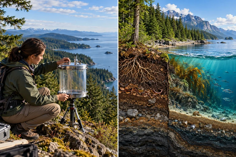Separate sampling-cylinder and coast/forest cutaway scenes distinguish a tagged-atom thought experiment from bulk reservoir redistribution. No generated molecule count or concentration color coding. Separate exact panel: A tagged carbon atom enters a reservoir alongside M/F; a separate bulk-pulse diagram shows atmosphere, ocean and land reservoirs exchanging carbon. Tracking one tagged carbon atom differs from tracking an added carbon pulse. M/F requires a defined stock, gross outflow and mixing assumptions; an added pulse redistributes among reservoirs over multiple timescales.

Tagged-atom exchange time differs from persistence of a bulk carbon perturbation.. Tracking one tagged carbon atom differs from tracking an added carbon pulse. M/F requires a defined stock, gross outflow and mixing assumptions; an added pulse redistributes among reservoirs over multiple timescales. 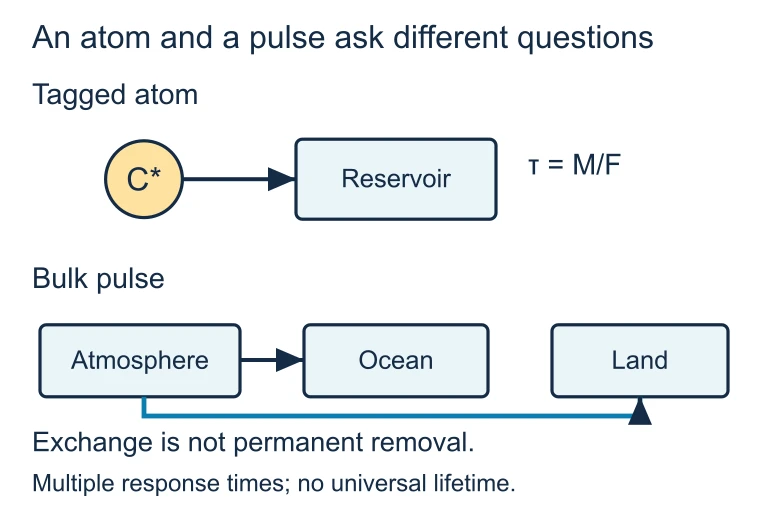Tracking one tagged carbon atom differs from tracking an added carbon pulse. M/F requires a defined stock, gross outflow and mixing assumptions; an added pulse redistributes among reservoirs over multiple timescales.

SECTION 6

Worked Example: Carbon Budget Calculation

The following worked example walks through a carbon budget analysis similar to what you might encounter on the AP Environmental Science exam. You will calculate the net change in atmospheric carbon and predict the resulting increase in CO₂ concentration.

Annual Atmospheric Carbon Budget

1
Step 1 — Identify the Fluxes

In a given year, the following approximate carbon fluxes are measured: Fossil fuel combustion adds 9.5 Gt C to the atmosphere. Land-use change (deforestation) adds 1.5 Gt C. The ocean absorbs 2.5 Gt C (net). The terrestrial biosphere absorbs 3.0 Gt C (net). We want to find the net annual change in atmospheric carbon.
2
Step 2 — Set Up the Budget Equation

ΔC_atm = (Sources) − (Sinks) = (Fossil fuels + Land-use change) − (Ocean uptake + Land uptake)
3
Step 3 — Substitute Values

ΔC_atm = (9.5 + 1.5) − (2.5 + 3.0) = 11.0 − 5.5

ΔC_atm = 5.5 Gt C/yr
4
Step 4 — Convert to ppm CO₂

Approximately 2.13 Gt C in the atmosphere corresponds to 1 ppm of CO₂. Therefore: Δppm = 5.5 Gt C ÷ 2.13 Gt C/ppm ≈ 2.58 ppm/yr.

Atmospheric CO₂ increases by approximately 2.6 ppm per year
5
Step 5 — Interpret the Result

This calculated value (~2.6 ppm/yr) closely matches the observed average annual increase recorded at Mauna Loa in recent years. The key insight is that roughly half (5.5 of 11.0 Gt C) of anthropogenic emissions remain in the atmosphere—the rest is absorbed by ocean and land sinks. This fraction is called the airborne fraction (~50%).

SECTION 7

Human Impacts on the Carbon Cycle

Human activities have perturbed the carbon cycle in ways that are unprecedented in geological history for their speed, if not their ultimate magnitude. The table below summarizes the major anthropogenic impacts, comparing the natural baseline flux with the human-caused perturbation, and identifying the environmental consequences that are most relevant to the AP Environmental Science exam.

Human Activity	Mechanism	Scale (Gt C/yr)	Key Environmental Consequence
Fossil fuel combustion	Oxidizes lithospheric C → atmospheric CO₂	~9.5	Enhanced greenhouse effect, global warming
Deforestation	Removes photosynthetic sinks; burning or decay releases stored biospheric C	~1.5	Reduced carbon sequestration, habitat loss, soil erosion
Cement production	Heating limestone (CaCO₃) releases CO₂	~1.5	Additional industrial CO₂ source
Agriculture (rice, cattle)	Anaerobic decomposition in paddies and enteric fermentation produce CH₄	~0.2 (as C in CH₄)	Methane is ~80× more potent GHG than CO₂ over 20 years
Excess CO₂ → ocean uptake	Additional CO₂ dissolves in ocean, forming carbonic acid	~2.5 (absorbed)	Ocean acidification: pH drop of ~0.1 since pre-industrial times harms coral reefs and shellfish

Major anthropogenic perturbations to the carbon cycle and their environmental consequences.

✦

KEY TAKEAWAY

The core problem is a rate mismatch: humans are transferring carbon from the slow geological cycle to the fast biological cycle at a rate the fast cycle cannot compensate for. Imagine filling a bathtub while the drain is only half open—the water level (atmospheric CO₂) will continue to rise until either the faucet is turned down (emission reductions) or the drain is widened (enhanced carbon sinks). Current natural sinks can only absorb about half of annual emissions, so the atmospheric carbon stock continues to grow.

SECTION 8

Feedback Loops & Connections to Other Cycles

The carbon cycle does not operate in isolation. It is coupled to other biogeochemical cycles and to Earth's climate system through feedback loops that can either amplify (positive feedback) or dampen (negative feedback) perturbations. Understanding these feedbacks is essential for predicting the trajectory of climate change and is a high-value topic on the AP exam.

Feedback Mechanism	Type	How It Works
Permafrost thaw	Positive	Warming thaws permafrost → decomposers release CO₂ and CH₄ from previously frozen organic matter → more warming
Reduced ocean CO₂ solubility	Positive	Warmer ocean absorbs less CO₂ → more CO₂ stays in atmosphere → more warming
CO₂ fertilization effect	Negative	Higher atmospheric CO₂ → increased photosynthesis rates (up to a point) → more carbon removed from atmosphere
Chemical weathering	Negative	Warmer, wetter climate increases chemical weathering of silicate rocks, consuming CO₂ from atmosphere → slow geological carbon removal over millions of years
Wildfire increase	Positive	Warming → drier conditions → more frequent/intense wildfires → rapid release of biospheric carbon → more warming

Key feedback loops connecting the carbon cycle to climate change.

The carbon cycle is also intimately connected to the nitrogen cycle (plants need nitrogen to photosynthesize, so nitrogen availability limits carbon uptake), the water cycle (evapotranspiration by plants links carbon fixation to water movement), and the phosphorus cycle (phosphorus is required for ATP and nucleic acids, which drive photosynthesis and respiration). On the AP exam, you should be prepared to explain how a perturbation in one cycle cascades through others. For example, excessive nitrogen fertilizer can stimulate algal growth (carbon uptake), but subsequent eutrophication depletes oxygen, kills aquatic organisms, and releases carbon through decomposition.

✦

KEY TAKEAWAY

Positive feedbacks in the carbon-climate system threaten to create a self-reinforcing cycle of warming, while negative feedbacks operate too slowly (chemical weathering takes millions of years) or have limited capacity (CO₂ fertilization saturates) to counterbalance anthropogenic emissions on human time scales. This asymmetry is why climate scientists emphasize the urgency of emission reductions.

SECTION 9

Practice Problems

Question 1: CONCEPTUAL

Which of the following best explains why burning fossil fuels disrupts the carbon cycle more significantly than cellular respiration, even though both processes release CO₂ into the atmosphere?

A. Fossil fuel combustion produces more CO₂ per molecule of reactant than cellular respiration does.
B. Fossil fuel combustion transfers carbon from a long-term geological reservoir to the atmosphere, while respiration recycles carbon that was recently fixed from the atmosphere by photosynthesis.
C. Cellular respiration only occurs in animals, whereas fossil fuel combustion is a global industrial process.
D. Fossil fuels release methane rather than CO₂, and methane is a more potent greenhouse gas.

Show answer (B)

Correct answer: B. The critical distinction is the source reservoir. Cellular respiration releases carbon that was recently removed from the atmosphere by photosynthesis (fast cycle), so there is no net addition. Fossil fuel combustion releases carbon that has been locked in the lithosphere for millions of years (slow cycle), adding new carbon to the atmosphere-biosphere system. Choice A is incorrect because per-molecule yield is not the relevant issue—the total amount matters, but more importantly the reservoir of origin. Choice C is incorrect because both plants and animals perform cellular respiration. Choice D is incorrect because burning fossil fuels primarily produces CO₂, not methane (though methane leaks are a concern).

Question 2: BASIC CALCULATION

The surface ocean contains approximately 900 Gt C, and the total flux of carbon into and out of the surface ocean is approximately 92 Gt C/yr. What is the approximate residence time of carbon in the surface ocean?

A. About 0.1 years
B. About 10 years
C. About 92 years
D. About 900 years

Show answer (B)

Correct answer: B. Using the residence time formula T = M / F: T = 900 Gt C ÷ 92 Gt C/yr ≈ 9.8 years, which rounds to about 10 years. Choice A (0.1 years) results from dividing the flux by the reservoir size (F/M), which is the inverse of residence time. Choice C (92 years) mistakes the flux value for the residence time. Choice D (900 years) mistakes the reservoir size for the residence time.

Question 3: INTERMEDIATE

Global ocean temperatures have risen by about 0.8 °C since pre-industrial times. A scientist notes that warmer water dissolves less CO₂. Which of the following correctly identifies the type of feedback loop this represents and its effect on atmospheric CO₂ levels?

A. Positive feedback loop; atmospheric CO₂ increases, further amplifying warming.
B. Positive feedback loop; atmospheric CO₂ decreases, further amplifying warming.
C. Negative feedback loop; atmospheric CO₂ increases, which then triggers greater ocean absorption.
D. Negative feedback loop; warming causes evaporation that removes CO₂ from the atmosphere.

Show answer (A)

Correct answer: A. This is a positive feedback loop: increased atmospheric CO₂ → warming → warmer ocean absorbs less CO₂ → even more CO₂ remains in the atmosphere → more warming. The initial perturbation is amplified, which is the hallmark of positive feedback. Choice B is incorrect because the mechanism described (reduced ocean absorption) would increase, not decrease, atmospheric CO₂. Choice C incorrectly identifies this as negative feedback; while higher CO₂ does increase the concentration gradient driving ocean absorption, the warming-induced reduction in solubility works against this, and the question specifically asks about the solubility effect. Choice D is incorrect because evaporation does not directly remove CO₂ from the atmosphere.

Question 4: APPLIED

4 pts

A research team wants to investigate whether a 500-hectare reforestation project acts as a net carbon sink. They measure the following data annually for three years: tree biomass carbon (via allometric equations and tree diameter measurements), soil organic carbon, litter carbon, and atmospheric CO₂ flux using eddy covariance towers. (a) Identify the independent variable, the dependent variable, and two variables that should be controlled or accounted for. (b) Describe how the team could determine whether the reforestation site is a net carbon sink or source. (c) Identify one potential source of error in this investigation and explain how it could affect results. (d) Explain why the team should continue monitoring for at least 10 years rather than relying on three years of data.

Show answer

Rubric (4 points): Point 1 (Variables): The independent variable is time since reforestation (or equivalently, tree age/stand maturity). The dependent variable is net carbon flux (or net ecosystem exchange of CO₂). Controlled/accounted variables include: tree species composition (should be uniform or recorded), climate variables (temperature, precipitation), prior land use history, or soil type. Point 2 (Methodology): The team should calculate the annual change in total ecosystem carbon (sum of tree biomass C + soil organic C + litter C). If the total carbon stored increases year over year—or if the eddy covariance towers show net downward CO₂ flux (atmosphere to ecosystem)—the site is a net carbon sink. If the reverse is true, it is a net source. Point 3 (Error): One potential source of error is that allometric equations used to estimate tree biomass may not be calibrated for the specific species or site conditions, leading to systematic overestimation or underestimation of carbon stored in tree biomass. Another acceptable answer: soil carbon measurements may miss deeper soil layers where decomposition releases CO₂, or eddy covariance data may be unreliable during calm nights. Any of these could cause the team to misclassify the site as a sink when it is neutral or even a source. Point 4 (Long-term monitoring): Three years of data may not capture interannual variability caused by climate fluctuations (e.g., drought years vs. wet years), disturbance events (fire, pest outbreaks), or the nonlinear trajectory of forest carbon uptake as trees mature. Young forests often accumulate carbon rapidly, but the rate may decline or even reverse as the stand ages or is affected by disturbance. Longer monitoring provides a more representative average and captures the trajectory of carbon storage over time.

Question 5: CRITICAL THINKING

4 pts

A country emits 1.2 Gt C per year from fossil fuel combustion and 0.3 Gt C per year from deforestation. Its remaining forests absorb 0.5 Gt C per year, and its adjacent ocean territory absorbs 0.2 Gt C per year. (a) Calculate the country's net annual carbon contribution to the atmosphere. (b) If the country's atmospheric carbon contribution is approximately 1/7 of the global net annual increase of 5.5 Gt C, calculate the country's percentage share of the global airborne carbon increase. Show your work. (c) The country proposes planting enough new forest to offset its entire net atmospheric contribution. Using the estimate that mature tropical forest sequesters approximately 5 tonnes of carbon per hectare per year, calculate the area of new forest needed (in hectares and km²). (d) Identify and explain one reason why the reforestation plan described in part (c) might not fully offset the country's emissions in practice.

Show answer

Rubric (4 points): Point 1 — Part (a): Net contribution = (Sources) − (Sinks) = (1.2 + 0.3) − (0.5 + 0.2) = 1.5 − 0.7 = 0.8 Gt C/yr net addition to the atmosphere. Point 2 — Part (b): Percentage share = (0.8 Gt C / 5.5 Gt C) × 100% ≈ 14.5% of the global net airborne carbon increase. (Note: 1/7 ≈ 14.3%, consistent with this calculation.) Point 3 — Part (c): To offset 0.8 Gt C/yr = 0.8 × 10⁹ tonnes C/yr at a rate of 5 tonnes C/ha/yr: Area = 0.8 × 10⁹ ÷ 5 = 1.6 × 10⁸ hectares = 160 million hectares. Converting: 160 million ha × (1 km²/100 ha) = 1.6 million km² (roughly the size of Alaska or Mongolia). Point 4 — Part (d): Acceptable reasons include: (1) Newly planted forests take decades to reach maturity and maximum carbon uptake rates—sequestration rates would be much lower than 5 t C/ha/yr in early years. (2) Forests are vulnerable to disturbances (fire, drought, pests, logging) that could release stored carbon back to the atmosphere. (3) As climate warms, forests in some regions may become net carbon sources due to increased respiration, drought stress, or wildfire. (4) The land area required (1.6 million km²) may not be physically or politically available. Any one of these, with a clear explanation of why it undermines full offset, earns the point.

SUMMARY

Summary: The Carbon Cycle

Summary

The carbon cycle describes the movement of carbon among four major reservoirs: the atmosphere (~870 Gt C), the biosphere (~2,000 Gt C), the hydrosphere (~38,000 Gt C), and the lithosphere (~75 million Gt C). Fluxes such as photosynthesis, respiration, ocean absorption, and volcanic outgassing transfer carbon between these pools. The fast (biological) carbon cycle operates on time scales of days to centuries, while the slow (geological) carbon cycle spans millions of years. Residence time (T = M / F) quantifies how long carbon stays in a reservoir.

Human activities—primarily fossil fuel combustion (~9.5 Gt C/yr) and deforestation (~1.5 Gt C/yr)—have shifted carbon from the slow geological cycle into the fast biological cycle at rates far exceeding natural fluxes. Roughly half of these emissions accumulate in the atmosphere (the airborne fraction ≈ 50%), driving the enhanced greenhouse effect and ocean acidification. Positive feedback loops (permafrost thaw, reduced ocean solubility, increased wildfire) threaten to amplify warming, while negative feedbacks (CO₂ fertilization, chemical weathering) operate too slowly or have limited capacity to fully compensate. Mastering the carbon cycle requires understanding reservoir sizes, flux magnitudes, residence times, feedback mechanisms, and the connections to Earth's nitrogen, phosphorus, and water cycles.