Sources of Pollution - AP Environmental Science

SECTION 1

Historical Context & Motivation

Pollution has accompanied human civilization since the earliest settlements concentrated waste in rivers and soils, but systematic recognition of pollution sources as a public health and ecological crisis did not emerge until the Industrial Revolution. The rapid combustion of coal in nineteenth-century London, the discharge of untreated industrial effluent into waterways, and the accumulation of chemical residues in agricultural soils collectively revealed that pollution could no longer be treated as a localized nuisance. By the mid-twentieth century, catastrophic events—from toxic smog episodes to rivers catching fire—compelled governments to classify pollution by its origin, distinguishing between identifiable discharge pipes and diffuse runoff from landscapes. This classification scheme became the regulatory backbone of modern environmental law and remains central to how the AP Environmental Science exam frames aquatic and terrestrial contamination.

1858 • The Great Stink of London

Raw sewage in the Thames produced such unbearable odors that Parliament was forced to fund a modern sewer system, marking one of the first large-scale governmental responses to water pollution.

1952 • London's Great Smog

A deadly smog event caused approximately 12,000 premature deaths. The disaster catalyzed the Clean Air Act of 1956 in the UK and demonstrated how stationary combustion sources could devastate air quality.

1969 • Cuyahoga River Fire

The Cuyahoga River in Cleveland, Ohio, caught fire due to accumulated industrial waste and oil slicks. The event galvanized public support for the U.S. Clean Water Act enacted in 1972.

1972 • U.S. Clean Water Act

The CWA formally codified the distinction between point sources and nonpoint sources of water pollution, establishing the National Pollutant Discharge Elimination System (NPDES) for regulating identifiable discharges.

1987 • CWA Amendments & Nonpoint Source Management

Section 319 of the amended Clean Water Act required states to develop nonpoint source pollution management programs, acknowledging that diffuse agricultural and urban runoff was the leading remaining cause of water quality impairment.

This historical trajectory reveals a key insight: controlling pollution requires first identifying where it originates. Whether a contaminant enters an ecosystem through a discrete pipe or across kilometers of agricultural landscape determines the regulatory tools, monitoring strategies, and remediation technologies that are most effective. The central question driving this lesson is therefore: How do we classify, trace, and manage the diverse sources through which pollutants enter aquatic and terrestrial systems?

SECTION 2

Core Principles & Definitions

At the foundation of pollution science lies a deceptively simple distinction: a point source is any single, identifiable, and often regulated location from which pollutants are discharged into the environment, such as a factory outfall pipe or a municipal wastewater treatment plant. A nonpoint source (NPS), by contrast, refers to pollution that enters water or soil from diffuse, spatially distributed origins—agricultural runoff carrying fertilizers across broad fields, urban stormwater washing oil and heavy metals off roads, or atmospheric deposition spreading mercury over a watershed. Understanding these core categories—and the factors that control pollutant fate once released—is essential for AP Environmental Science.

Point Sources

Discrete, identifiable discharge locations such as industrial outfalls, sewage treatment plants, and confined animal feeding operations (CAFOs). These are typically regulated under permit systems like NPDES.

Nonpoint Sources

Diffuse, landscape-scale pollution from agricultural runoff, urban stormwater, construction sites, and atmospheric deposition. NPS pollution is the leading cause of water quality impairment in the United States.

Primary vs. Secondary Pollutants

Primary pollutants (e.g., SO₂, particulate matter) are emitted directly from a source. Secondary pollutants (e.g., tropospheric O₃, acid rain) form through chemical reactions in the environment from precursor emissions.

Bioaccumulation & Biomagnification

Persistent pollutants such as DDT, PCBs, and methylmercury accumulate in organisms (bioaccumulation) and increase in concentration at higher trophic levels (biomagnification), amplifying harm far from the original source.

Pollutant Fate & Transport

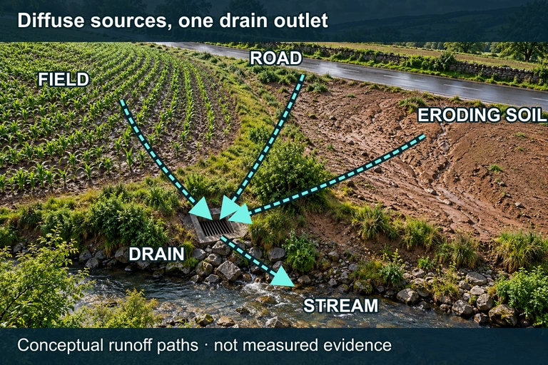Once released, pollutants undergo transport (advection, diffusion), transformation (photolysis, biodegradation), and partitioning among air, water, soil, and biota. These processes determine exposure levels and ecological impact.

A conceptual field, road and eroding soil sit above a drain and stream. Dashed arrows from the three land surfaces converge on the drain; a fourth arrow reaches the stream. Rainfall can carry pollution from diffuse field, road and eroding-soil sources through a connected drain network to one outlet. A concentrated final conduit does not make every upstream source a point source. The routes are conceptual, not measured.

✦

KEY TAKEAWAY

Think of point sources like a leaking faucet in your kitchen—you can see exactly where the water drips and fix it with a wrench. Nonpoint source pollution is more like condensation forming on every cold surface in the house simultaneously: there is no single leak to repair, so you must change the overall conditions (ventilation, insulation) to address it. In environmental policy, this analogy explains why point sources were regulated first (straightforward to monitor and control), while nonpoint source management requires broader land-use planning, best management practices, and incentive programs.

SECTION 3

Visual Explanation: Point vs. Nonpoint Source Diagram

This diagram contrasts point sources (left, solid arrows from identifiable discharge locations) with nonpoint sources (right, dashed arrows representing diffuse runoff). Both ultimately impact receiving water bodies and can infiltrate into soil and groundwater. Note the regulatory distinction at the bottom: point sources are controlled through permit systems, while nonpoint sources require best management practices (BMPs) and broader land-use strategies.

The diagram above illustrates the fundamental spatial distinction that drives environmental regulation. On the left side, a factory outfall and a wastewater treatment plant each discharge through a single pipe into the receiving water body—these are classic point sources whose flow rate, chemical composition, and temperature can be monitored at a single location. On the right, agricultural runoff and urban stormwater enter the water body along extended stretches of shoreline, carried by sheet flow and storm drains across broad areas. Because no single pipe can be identified, these nonpoint sources are far more difficult to monitor, attribute, and regulate. Both categories of pollution ultimately affect aquatic and terrestrial systems, infiltrating soil and contaminating groundwater reserves. Understanding this visual framework is the first step toward mastering the pollution questions on the AP Environmental Science exam.

SECTION 4

Mechanisms of Pollution Transport & Transformation

Once pollutants are released from either point or nonpoint sources, their environmental impact depends on how they are transported and transformed. Several interconnected mechanisms govern pollutant fate in aquatic and terrestrial systems, and the AP exam frequently tests your ability to distinguish among them.

Oxygen Demand & Eutrophication

When organic pollutants—from sewage, food processing, or animal waste—enter a water body, aerobic bacteria decompose them and consume dissolved oxygen (DO). The biochemical oxygen demand (BOD) quantifies this oxygen consumption. High BOD values indicate heavy organic loading and the potential for hypoxic or anoxic conditions. Similarly, excess nutrients (nitrogen and phosphorus) from agricultural fertilizers and wastewater trigger eutrophication—the rapid growth of algae whose subsequent decomposition further depletes dissolved oxygen, creating dead zones where aquatic organisms cannot survive.

BOD CONCEPTUAL MODEL

DO_deficit = DO_saturation − DO_measured

Where DO_saturation is the maximum dissolved oxygen a water body can hold at a given temperature, and DO_measured is the actual concentration observed. The greater the deficit, the higher the organic pollution load.

Bioaccumulation & Biomagnification

Persistent, lipophilic pollutants such as DDT, PCBs, and methylmercury resist metabolic breakdown and dissolve readily in fatty tissues. An organism absorbs these chemicals faster than it can excrete them, leading to bioaccumulation over its lifetime. When a predator consumes many contaminated prey organisms, the pollutant concentration magnifies at each successive trophic level—a process called biomagnification. This mechanism explains why top predators such as bald eagles and tuna accumulate the highest contaminant burdens even though ambient water concentrations may be extremely low.

BIOMAGNIFICATION FACTOR

BMF = C_predator / C_prey

Where C_predator is the concentration of a contaminant in the predator's tissues and C_prey is the concentration in prey tissues. A BMF > 1 indicates biomagnification is occurring.

Atmospheric Deposition & Acid Rain

Air pollutants released from power plants, vehicles, and industrial facilities undergo atmospheric transport and chemical transformation. Sulfur dioxide (SO₂) and nitrogen oxides (NO_x) are primary pollutants that react with water vapor and oxygen to form sulfuric and nitric acids—secondary pollutants that fall as acid rain or dry deposition. These mechanisms connect distant emission sources to aquatic and terrestrial damage hundreds of kilometers downwind, blurring the boundary between point and nonpoint classification.

ACID RAIN FORMATION (SIMPLIFIED)

SO₂ + H₂O → H₂SO₃ (further oxidized to H₂SO₄)

Sulfur dioxide emitted from coal-fired power plants dissolves in atmospheric moisture to form sulfurous acid, which is further oxidized to sulfuric acid (H₂SO₄), lowering precipitation pH well below the natural baseline of ≈ 5.6.

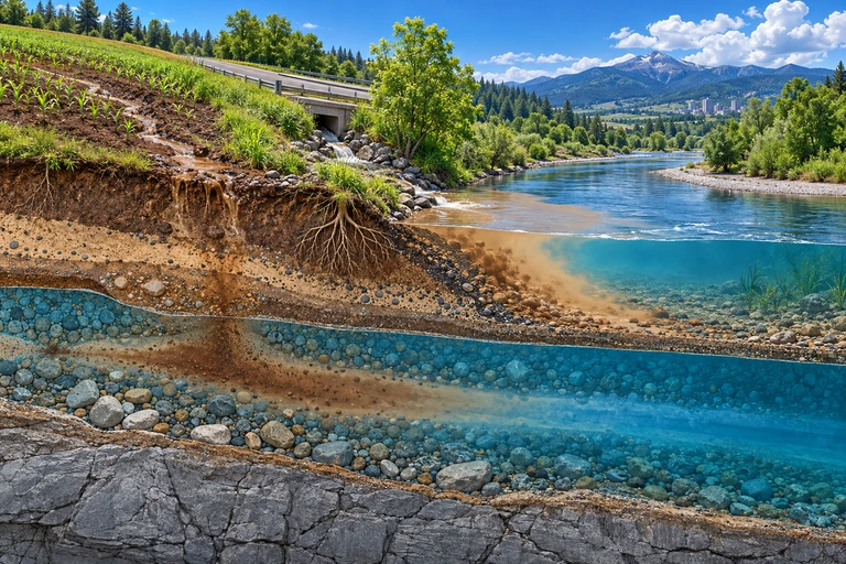A field,road and river above a soil and groundwater cutaway showing several transport contexts. Dissolved pollutants can move with groundwater, while adsorbed pollutants may travel with sediment. Chemical form affects transport and exposure; intake, absorbed dose and tissue concentration are different quantities.

Dissolved and sediment-bound differ. Dissolved pollutants can move with groundwater, while adsorbed pollutants may travel with sediment. Chemical form affects transport and exposure; intake, absorbed dose and tissue concentration are different quantities. 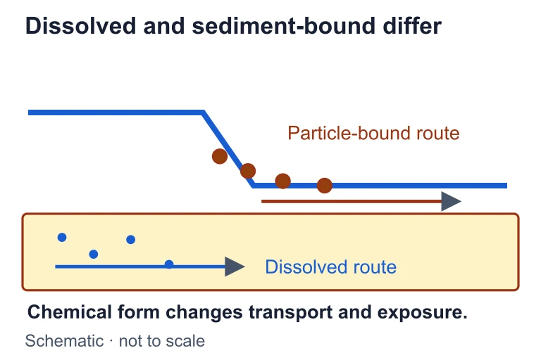Dissolved pollutants can move with groundwater, while adsorbed pollutants may travel with sediment. Chemical form affects transport and exposure; intake, absorbed dose and tissue concentration are different quantities.

SECTION 5

Detailed Classification of Pollution Sources

The AP Environmental Science curriculum organizes pollution sources along multiple axes: by medium (air, water, soil), by spatial pattern (point vs. nonpoint), and by the type of pollutant released (chemical, biological, physical, thermal). The following diagram and table provide a comprehensive classification framework that integrates these dimensions.

This hierarchical diagram organizes pollution sources first by environmental medium (air, water, soil), then subdivides each into point and nonpoint categories with specific examples. The bottom panel classifies pollutant types: chemical, biological, physical, and thermal.

Pollution Source Type	Examples	Key Pollutants	Primary Medium Affected
Industrial point source	Factory discharge pipes, refineries, smelters	Heavy metals (Pb, Hg, Cd), organic solvents, thermal effluent	Water, Air
Municipal point source	Wastewater treatment plants, sewage overflows	Pathogens, nutrients (N, P), pharmaceuticals, BOD	Water
Agricultural nonpoint	Cropland runoff, irrigated fields, livestock operations	Nitrates, phosphates, pesticides, sediment, pathogens	Water, Soil
Urban nonpoint	Parking lots, roads, construction sites, lawns	Oil, heavy metals, sediment, plastics, bacteria	Water, Soil
Atmospheric (mobile)	Vehicles, aircraft, shipping	CO, NOₓ, VOCs, PM₂.₅, CO₂	Air
Mining / extraction	Acid mine drainage, tailings ponds, hydraulic fracturing	Sulfuric acid, heavy metals, sediment, fracking fluids	Water, Soil

Summary of major pollution source categories tested on the AP Environmental Science exam

SECTION 6

Worked Example: Identifying Sources & Calculating Impact

The following worked example mirrors the type of scenario-based analysis you will encounter on the AP Environmental Science exam. It integrates source identification with a quantitative assessment of pollutant loading.

Nutrient Loading from Mixed Sources into a Lake

1
Step 1 — Identify the Scenario

A lake receives water from three inputs: (1) a municipal wastewater treatment plant (WWTP) that discharges 5.0 × 10⁶ liters per day with a phosphorus concentration of 2.0 mg/L; (2) agricultural runoff from surrounding farms estimated at 1.2 × 10⁷ liters per day with a phosphorus concentration of 0.4 mg/L; and (3) urban stormwater at 3.0 × 10⁶ liters per day with a phosphorus concentration of 0.3 mg/L. Determine the daily phosphorus load from each source and identify the largest contributor.
2
Step 2 — Classify Each Source

The WWTP is a point source because it discharges through an identifiable pipe under an NPDES permit. The agricultural runoff and urban stormwater are both nonpoint sources because they originate from diffuse, landscape-scale flows rather than a single discharge point.
3
Step 3 — Calculate Phosphorus Load for Each Source

Pollutant load (mass/time) = flow rate × concentration. For the WWTP: Load = 5.0 × 10⁶ L/day × 2.0 mg/L = 1.0 × 10⁷ mg/day = 10.0 kg/day. For agricultural runoff: Load = 1.2 × 10⁷ L/day × 0.4 mg/L = 4.8 × 10⁶ mg/day = 4.8 kg/day. For urban stormwater: Load = 3.0 × 10⁶ L/day × 0.3 mg/L = 9.0 × 10⁵ mg/day = 0.9 kg/day.

WWTP = 10.0 kg P/day | Ag. runoff = 4.8 kg P/day | Urban stormwater = 0.9 kg P/day
4
Step 4 — Determine Total Load and Percent Contribution

Total daily phosphorus load = 10.0 + 4.8 + 0.9 = 15.7 kg/day. Percent contributions: WWTP = (10.0 / 15.7) × 100 ≈ 63.7%. Agricultural runoff = (4.8 / 15.7) × 100 ≈ 30.6%. Urban stormwater = (0.9 / 15.7) × 100 ≈ 5.7%.

The point source (WWTP) contributes ≈ 63.7% of total phosphorus loading, making it the single largest contributor despite nonpoint sources collectively accounting for ≈ 36.3%.
5
Step 5 — Interpret & Recommend

Although the WWTP contributes the majority of phosphorus, upgrading its treatment technology (e.g., adding chemical phosphorus removal) addresses only the point source fraction. Achieving water quality targets likely requires a combined strategy: upgrading the WWTP to reduce discharge concentrations below 0.5 mg/L while simultaneously implementing agricultural BMPs (buffer strips, cover crops, nutrient management plans) and urban stormwater controls (rain gardens, permeable pavement). This integrated approach is a hallmark of Total Maximum Daily Load (TMDL) planning, which the AP exam frequently references.

SECTION 7

Regulatory Approaches: Strengths & Limitations

Effective pollution control hinges on matching the right regulatory tool to the source type. The U.S. regulatory framework offers a useful case study because it employs fundamentally different strategies for point versus nonpoint sources—a distinction the AP exam expects you to analyze critically.

Feature	Point Source Regulation	Nonpoint Source Management
Primary mechanism	NPDES permits with enforceable discharge limits (technology-based and water-quality-based standards)	Voluntary BMPs, cost-share incentive programs (CWA §319), and state-level management plans
Monitoring	Direct sampling at the discharge point; continuous electronic monitoring possible	Watershed-scale modeling, land-use surveys, ambient water quality monitoring
Strengths	High accountability; clear legal liability; dramatic reductions in industrial and municipal discharges since 1972	Addresses the largest remaining source of water quality impairment; flexible, site-specific solutions
Limitations	Does not address diffuse runoff; compliance costs can be high for small municipalities; combined sewer overflows remain problematic	Largely voluntary and underfunded; difficult to measure effectiveness; politically challenging to impose land-use restrictions on agriculture
Key legislation	Clean Water Act §402 (NPDES); Clean Air Act (NSR permits for stationary sources)	CWA §319; Farm Bill conservation programs (EQIP, CRP); TMDL framework

Comparison of regulatory approaches for point and nonpoint pollution sources

✦

KEY TAKEAWAY

The regulatory asymmetry between point and nonpoint sources is analogous to the difference between treating a patient with a known bacterial infection (prescribe a targeted antibiotic) versus preventing chronic disease across an entire population (require systemic changes in diet, exercise, and environment). Both are essential, but the latter demands broader societal coordination and is much harder to enforce. On the AP exam, expect questions that ask you to evaluate the effectiveness of NPDES permits versus voluntary BMP programs or to propose TMDL allocations that distribute pollution reduction responsibilities between point and nonpoint sources.

SECTION 8

Connections to Advanced Environmental Topics

Understanding pollution sources provides the foundation for several advanced topics you will encounter later in the AP Environmental Science curriculum and in collegiate environmental science coursework. The table below connects source-level concepts to their broader implications in environmental policy, toxicology, and sustainability.

Foundational Concept	Advanced Connection
Point vs. nonpoint classification	TMDL development: allocating maximum pollutant loads across a watershed by assigning waste load allocations (WLAs) to point sources and load allocations (LAs) to nonpoint sources
Biomagnification of persistent pollutants	Environmental toxicology: dose-response models, LD₅₀ testing, endocrine disruption studies, and the Stockholm Convention on Persistent Organic Pollutants (POPs)
Eutrophication from nutrient loading	Dead zone formation (e.g., Gulf of Mexico hypoxia); integrated watershed management; precision agriculture to minimize fertilizer overuse
Primary and secondary air pollutants	Tropospheric ozone formation, photochemical smog modeling, cap-and-trade systems (SO₂ Acid Rain Program), and climate change mitigation via CO₂ emission controls
Pollutant fate and transport	Environmental modeling (e.g., Streeter-Phelps BOD/DO sag curve), Superfund site remediation, and life cycle assessment (LCA) in industrial ecology

How foundational pollution source concepts connect to advanced environmental topics

The transition from source identification to systems-level analysis represents the intellectual arc of AP Environmental Science. While this lesson focuses on recognizing and classifying where pollutants originate, subsequent units address how those pollutants interact with biogeochemical cycles, affect ecosystem services, and drive policy debates about environmental justice—the observation that pollution sources are disproportionately located near low-income communities and communities of color. Mastering source classification now will equip you to engage critically with these more complex, interdisciplinary questions.

SECTION 9

Practice Problems

Question 1: CONCEPTUAL

A farmer applies nitrogen fertilizer to a 200-hectare cornfield. After a rainstorm, monitoring stations downstream detect elevated nitrate concentrations in the river. Which of the following best classifies this pollution?

A. Point source pollution, because the farmer is the identifiable origin
B. Nonpoint source pollution, because the nitrate enters the river from diffuse runoff across the landscape
C. Secondary pollution, because the nitrate was chemically transformed from the fertilizer
D. Thermal pollution, because the rainstorm alters the temperature of the river

Show answer (B)

The correct answer is B. Agricultural runoff is the classic example of nonpoint source (NPS) pollution because it enters the water body from diffuse, distributed overland flow rather than from a single identifiable discharge pipe. Choice A is incorrect because, although the farmer is identifiable, the pollution does not originate from a single discrete discharge point—it washes across an entire 200-hectare field. Choice C is incorrect because the nitrate in this case is the fertilizer compound itself entering the waterway, not a product of atmospheric chemical transformation (which would define a secondary pollutant like ozone or acid rain). Choice D is incorrect because thermal pollution refers specifically to elevated water temperatures from industrial cooling water discharges, not from rainstorm events.

Question 2: BASIC CALCULATION

A factory discharges 8.0 × 10⁵ L/day of wastewater containing 5.0 mg/L of lead (Pb). What is the daily lead load discharged into the receiving river?

A. 0.4 kg/day
B. 4.0 kg/day
C. 40 kg/day
D. 400 kg/day

Show answer (B)

The correct answer is B. Load = flow rate × concentration = 8.0 × 10⁵ L/day × 5.0 mg/L = 4.0 × 10⁶ mg/day. Converting to kilograms: 4.0 × 10⁶ mg ÷ 10⁶ mg/kg = 4.0 kg/day. Choice A (0.4 kg/day) results from an error in the exponent during multiplication or an incorrect unit conversion. Choice C (40 kg/day) is off by a factor of 10, likely from misreading the flow rate as 8.0 × 10⁶ L/day. Choice D (400 kg/day) is off by two orders of magnitude, suggesting a fundamental unit conversion error.

Question 3: INTERMEDIATE

Mercury concentrations in a lake ecosystem are measured as follows: water = 0.001 mg/L, phytoplankton = 0.05 mg/kg, zooplankton = 0.5 mg/kg, small fish = 5.0 mg/kg, and large predatory fish = 50 mg/kg. Which of the following correctly identifies the process and the biomagnification factor (BMF) between small fish and large predatory fish?

A. Bioaccumulation; BMF = 10
B. Biomagnification; BMF = 10
C. Biomagnification; BMF = 50
D. Bioaccumulation; BMF = 50

Show answer (B)

The correct answer is B. The increase in mercury concentration from one trophic level to the next is biomagnification, and the BMF between small fish and large predatory fish = C_predator / C_prey = 50 mg/kg ÷ 5.0 mg/kg = 10. Choice A incorrectly labels the process as bioaccumulation; bioaccumulation describes pollutant accumulation within a single organism over its lifetime, not the increase across trophic levels. Choice C calculates BMF incorrectly, likely dividing 50 by 1 (confusing the concentration value with the BMF). Choice D combines both errors—wrong process name and wrong BMF value.

Question 4: APPLIED

4 pts

A state environmental agency is developing a TMDL for phosphorus in a lake that can assimilate no more than 25 kg of phosphorus per day without triggering eutrophication. Current daily loads are: wastewater treatment plant (point source) = 12 kg/day, agricultural runoff (nonpoint source) = 10 kg/day, urban stormwater (nonpoint source) = 5 kg/day, and a margin of safety = 3 kg/day. Design an investigation to determine which agricultural BMPs are most effective at reducing phosphorus loading to meet the TMDL target. Parts: (a) State a testable hypothesis about BMP effectiveness. (b) Describe an experimental design including independent variable, dependent variable, control, and at least two treatments. (c) Identify one potential confounding variable and explain how to control for it. (d) Explain how the results of this investigation could be applied to the TMDL allocation.

Show answer

Point-by-point rubric: (a) 1 point — Hypothesis: A clear, testable hypothesis is stated, e.g., 'Vegetated riparian buffer strips of at least 10 meters will reduce phosphorus concentrations in agricultural runoff by at least 40% compared to fields without buffer strips.' The hypothesis must include the independent variable (BMP type or buffer width), the expected direction of change, and the dependent variable (phosphorus concentration or load). (b) 1 point — Experimental Design: The student describes an experiment with: an independent variable (type of BMP, e.g., 10 m buffer strip vs. cover crops vs. no-till farming); a dependent variable (phosphorus concentration in runoff collected at the field edge, measured in mg/L); a control (field plots with no BMP applied, representing current practices); and at least two treatment groups. Replication (multiple plots per treatment) should be mentioned. Runoff samples should be collected after rain events and analyzed for dissolved and particulate phosphorus. (c) 1 point — Confounding Variable: One confounding variable is identified (e.g., differences in soil type, slope, rainfall intensity, or pre-existing soil phosphorus levels between plots) with a clear strategy for control (e.g., randomizing treatment assignments across plots with similar slope and soil type, or using a randomized block design to account for spatial variability). (d) 1 point — TMDL Application: The student explains that the investigation results would quantify the percent phosphorus reduction achievable by each BMP. The current total load is 27 kg/day (12 + 10 + 5), but the TMDL target is 25 kg/day minus the 3 kg/day margin of safety = 22 kg/day of allowable loading. This requires a total reduction of 5 kg/day. If buffer strips reduce agricultural loading by 40%, the agricultural contribution drops from 10 to 6 kg/day, achieving a 4 kg/day reduction. The remaining 1 kg/day reduction could be allocated to the WWTP through enhanced phosphorus removal. This demonstrates how BMP effectiveness data informs the allocation of load reductions between point and nonpoint sources in a TMDL.

Question 5: CRITICAL THINKING

4 pts

A researcher collects the following data from three sampling stations along a river downstream of both a wastewater treatment plant (WWTP, point source at km 0) and a large agricultural region (nonpoint source, km 5–15): Station A (km 2): Dissolved oxygen = 4.2 mg/L, Nitrate = 3.8 mg/L, Fecal coliform = 850 CFU/100 mL Station B (km 10): Dissolved oxygen = 6.8 mg/L, Nitrate = 12.5 mg/L, Fecal coliform = 120 CFU/100 mL Station C (km 20): Dissolved oxygen = 5.1 mg/L, Nitrate = 9.0 mg/L, Fecal coliform = 200 CFU/100 mL Parts: (a) Identify which pollutant parameter is most strongly associated with the point source and explain your reasoning using the data. (b) Identify which pollutant parameter is most strongly associated with the nonpoint source and explain your reasoning. (c) Explain the dissolved oxygen pattern across the three stations, referencing specific pollution processes. (d) Propose one management strategy for each source type (point and nonpoint) that would improve water quality at Station C, and justify each.

Show answer

Point-by-point rubric: (a) 1 point — Point Source Pollutant: Fecal coliform is most strongly associated with the WWTP point source. The data show the highest fecal coliform count (850 CFU/100 mL) at Station A (km 2), which is closest to the WWTP discharge at km 0. Fecal coliform decreases sharply downstream (120 at km 10, 200 at km 20), consistent with dilution and die-off patterns expected from a point source discharge. Municipal wastewater is a primary source of fecal bacteria. (b) 1 point — Nonpoint Source Pollutant: Nitrate is most strongly associated with the agricultural nonpoint source. Nitrate is lowest at Station A (3.8 mg/L) upstream of the agricultural region, peaks at Station B (12.5 mg/L) in the middle of the agricultural zone (km 5–15), and remains elevated at Station C (9.0 mg/L) downstream. This spatial pattern—increasing concentration along the stretch where agricultural runoff enters—is characteristic of nonpoint source loading. Fertilizer application on farms is a major source of nitrate in surface waters. (c) 1 point — DO Pattern Explanation: Dissolved oxygen is lowest at Station A (4.2 mg/L) because the WWTP's organic-rich effluent creates high BOD, and aerobic decomposition of this organic matter consumes dissolved oxygen near the discharge point. By Station B (km 10), DO has recovered to 6.8 mg/L as the river has reaerated through atmospheric exchange and turbulent mixing, and the BOD load from the WWTP has been partially consumed. At Station C (km 20), DO drops slightly to 5.1 mg/L, likely because algal growth stimulated by agricultural nitrate loading is beginning to decompose, creating localized oxygen demand—an early indicator of eutrophication from the nonpoint source nutrient input. (d) 1 point — Management Strategies: For the point source (WWTP): Upgrade to tertiary treatment with UV disinfection or chlorination/dechlorination to reduce fecal coliform counts in the effluent before discharge, ensuring compliance with NPDES permit limits for pathogens. This is justified because the data show the WWTP is the dominant source of fecal contamination. For the nonpoint source (agriculture): Implement riparian buffer zones along the river through the agricultural corridor (km 5–15) to intercept nitrate-laden runoff before it reaches the water body, combined with precision nutrient management plans to reduce fertilizer application to agronomic rates. This is justified because the data show nitrate peaks in the agricultural zone, and vegetated buffers have been shown to reduce nitrate loading by 50–80% through denitrification and plant uptake.

SUMMARY

Summary

Pollution sources are classified primarily as point sources—single, identifiable discharge locations like factory outfalls and wastewater treatment plants regulated through NPDES permits—and nonpoint sources—diffuse, landscape-scale inputs such as agricultural runoff and urban stormwater managed through voluntary best management practices (BMPs). Pollutants are further categorized as primary (emitted directly) or secondary (formed through environmental reactions), and their impact is amplified through mechanisms like bioaccumulation, biomagnification, and eutrophication.

Quantitative tools—pollutant loading calculations (Load = flow × concentration), BOD measurements, and biomagnification factors—allow scientists and regulators to trace pollution to its origin and allocate reduction targets through Total Maximum Daily Load (TMDL) plans. For the AP exam, remember that controlling pollution effectively requires addressing both point sources (through permit systems and technology upgrades) and nonpoint sources (through land-use planning, buffer zones, and nutrient management), and that environmental justice considerations demand attention to the disproportionate siting of pollution sources near vulnerable communities.