Noise Pollution - AP Environmental Science

SECTION 1

Historical Context & Motivation

Although humans have complained about unwanted sound for millennia—ancient Rome enacted daytime bans on iron-wheeled chariots to protect sleep—noise pollution only became a subject of formal scientific and regulatory study during the Industrial Revolution, when steam engines, textile mills, and rail networks dramatically amplified the acoustic environment of cities. Prolonged exposure to industrial noise was linked to hearing loss among factory workers as early as the 1830s, yet decades passed before governments treated noise as a genuine environmental contaminant rather than a mere nuisance. The twentieth century's rapid mechanization of transportation and urbanization thrust the issue into public health discourse, culminating in landmark legislation that placed sound alongside particulates, ozone, and heavy metals as a regulated pollutant.

1713 • Ramazzini's Occupational Noise Study

Italian physician Bernardino Ramazzini documented hearing loss in coppersmiths and other tradespeople, providing one of the earliest medical accounts linking occupational noise to human health effects.

1972 • U.S. Noise Control Act

Congress declared that inadequately controlled noise endangers the health and welfare of the American people, tasking the EPA with establishing noise emission standards for major sources such as transportation, construction, and electrical equipment.

1999 • WHO Guidelines on Community Noise

The World Health Organization published comprehensive guidelines establishing health-based noise thresholds—for example, a 55 dB daytime limit outdoors—shifting the conversation toward evidence-based exposure standards for cardiovascular, psychological, and cognitive effects.

2011 • EU Environmental Noise Directive Progress

European member states produced strategic noise maps covering all major agglomerations and transport corridors, enabling systematic action plans and raising awareness that more than 100 million EU residents were exposed to road-traffic noise above recommended levels.

2018 • WHO Environmental Noise Guidelines for Europe

Updated WHO guidelines recommended even stricter limits (e.g., road-traffic noise below 53 dB Lden) and for the first time included strong recommendations for reducing wind-turbine and leisure noise, reflecting growing evidence of non-auditory health impacts.

Despite this regulatory history, noise pollution remains one of the most underappreciated environmental stressors. The central question the AP Environmental Science curriculum asks is: How does anthropogenic noise interact with human health and ecological systems, and what strategies can meaningfully mitigate its impacts? Answering that question requires understanding the physics of sound measurement, the biological pathways of noise-induced harm, and the policy tools available to manage exposure.

SECTION 2

Core Principles & Definitions

At its most fundamental level, noise pollution is unwanted or harmful sound that disrupts normal activities, degrades quality of life, or damages health. Sound itself is a longitudinal pressure wave propagating through a medium—usually air—and is characterized by its frequency (measured in hertz, Hz) and amplitude (measured in decibels, dB). The human ear can perceive frequencies roughly from 20 Hz to 20,000 Hz, and sounds below 0 dB are essentially inaudible to most people, while sounds above 85 dB sustained over eight hours can cause permanent hearing damage.

Decibel Scale (dB)

A logarithmic scale that expresses sound intensity relative to the threshold of human hearing (10⁻¹² W/m²). Every 10 dB increase represents a tenfold increase in sound intensity; every 3 dB increase roughly doubles it.

Point & Non-Point Sources

Point sources emit noise from an identifiable location (e.g., a factory or airport runway). Non-point sources are diffuse, such as aggregate urban traffic. Regulation strategies differ for each category.

Acute vs. Chronic Exposure

Acute exposure—a single blast or explosion—can rupture eardrums instantly. Chronic exposure to moderate noise (60–80 dB) over months or years leads to cardiovascular stress, sleep disruption, and cognitive impairment.

Ecological Noise Effects

Wildlife relies on acoustic signals for mating, predator avoidance, and territory defense. Anthropogenic noise masks these signals, reducing reproductive success and altering species distributions in both terrestrial and marine habitats.

✦

KEY TAKEAWAY

Think of the decibel scale the way seismologists think of the Richter scale: both are logarithmic, so a seemingly small numerical jump (say, from 70 dB to 80 dB) actually represents a tenfold increase in intensity. This is precisely why environmental scientists are concerned about incremental increases in ambient noise: what sounds trivially louder to the ear may be imposing dramatically greater energy on biological tissues.

SECTION 3

Visual Explanation — The Decibel Spectrum

The decibel spectrum from the threshold of hearing (0 dB) to levels that cause immediate pain (125+ dB). The 85 dB damage threshold is the key regulatory benchmark; sustained exposure above this level causes irreversible noise-induced hearing loss (NIHL).

The diagram above situates everyday sound sources along the decibel continuum and maps them to three health-effect zones. Notice that the transition from green (safe) to amber (caution) occurs around 70 dB—roughly the level of a busy restaurant—while the red (danger) zone begins at the 85 dB occupational exposure limit established by NIOSH. Because the decibel scale is logarithmic, the sound energy at 85 dB is roughly 30 times greater than at 70 dB, even though the numerical difference appears modest. For AP Environmental Science, it is essential to understand that chronic exposure to levels in the caution zone already elevates risks of cardiovascular disease, hypertension, and cognitive impairment—effects that accumulate silently over years, much like the health consequences of long-term air-pollutant exposure.

SECTION 4

Mathematical Framework — The Decibel Scale

Sound intensity is the power per unit area carried by a sound wave, measured in watts per square meter (W/m²). Because the range of intensities the human ear can perceive spans roughly twelve orders of magnitude, scientists use the decibel (dB) scale—a logarithmic compression that makes comparing vastly different intensities tractable. The AP exam expects you to interpret and apply the decibel formula, understand the reference intensity, and translate decibel changes into real-world intensity ratios.

SOUND INTENSITY LEVEL

β = 10 × log₁₀(I / I₀)

β = sound intensity level in decibels (dB); I = measured sound intensity (W/m²); I₀ = reference intensity = 10⁻¹² W/m² (threshold of human hearing); log₁₀ = common (base-10) logarithm.

INTENSITY RATIO FROM DECIBEL CHANGE

I₂ / I₁ = 10^(Δβ / 10)

Δβ = change in decibel level (dB); I₂/I₁ = ratio of the two sound intensities. A 10 dB increase means intensity multiplied by 10; a 3 dB increase means intensity roughly doubled.

INVERSE SQUARE LAW (SOUND IN OPEN AIR)

I = P / (4πr²)

I = sound intensity at distance r from a point source (W/m²); P = acoustic power output (W); r = distance from the source (m). Sound intensity decreases with the square of the distance; doubling distance reduces intensity by a factor of 4 (≈ 6 dB reduction).

✦

KEY TAKEAWAY

The most commonly tested quantitative relationship on the APES exam is that a 10 dB increase corresponds to a 10× increase in sound intensity. Meanwhile, the inverse square law tells us that simply doubling your distance from a noise source drops intensity by about 6 dB—a practical principle used in buffer-zone planning around airports and highways.

SECTION 5

Sources, Pathways, and Ecological Effects

Noise pollution originates from a wide array of anthropogenic activities, and its effects propagate through both atmospheric and aquatic media. The AP exam commonly tests your ability to identify major noise sources, describe their ecological consequences, and distinguish between human-health and wildlife impacts. The diagram below maps the primary source categories to the organisms and systems they affect.

A flowchart mapping the four major source categories of noise pollution through their transmission pathways (atmospheric, aquatic, and ground vibration) to both human health effects and ecological effects. Lines connecting boxes indicate documented causal pathways.

Source Category	Typical dB Range	Primary Ecological Impact
Road traffic	70 – 85 dB	Habitat fragmentation for terrestrial species; avoidance of roadside zones reduces effective habitat area
Aircraft	90 – 130 dB (near runway)	Bird nest abandonment; reduced breeding success near airports
Naval sonar	Up to 235 dB underwater	Cetacean disorientation, mass strandings, disrupted echolocation in dolphins and whales
Construction / industry	80 – 110 dB	Displacement of sensitive species; elevated cortisol levels in wildlife in adjacent areas

Major noise pollution sources, their typical decibel ranges, and documented ecological impacts

Two similar songbirds face one another across a road. A hypothetical time-frequency diagram marks traffic below3kHz and a call spanning2–5kHz, with a2–3kHz overlap. Traffic can mask portions of an animal call when their frequency and time ranges overlap within the listener’s sensitivity. Detectability depends on the signal, background noise and receiver.

Hypothetical acoustic masking bands. Traffic can mask portions of an animal call when their frequency and time ranges overlap within the listener’s sensitivity. Detectability depends on the signal, background noise and receiver. 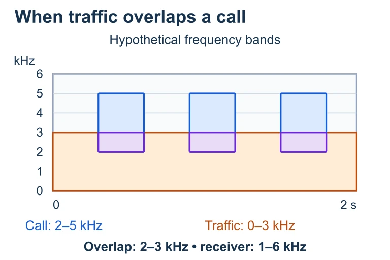Traffic can mask portions of an animal call when their frequency and time ranges overlap within the listener’s sensitivity. Detectability depends on the signal, background noise and receiver.

SECTION 6

Worked Example — Applying the Decibel Scale and Inverse Square Law

A construction site generates sound at an intensity of 10⁻³ W/m² at a distance of 15 m from the jackhammer. A residential neighborhood begins 120 m from the source. Calculate the sound level in decibels at the construction site (15 m) and at the neighborhood (120 m), then determine whether the neighborhood level exceeds the WHO daytime guideline of 55 dB.

Noise Impact Assessment

1
Step 1 — Calculate dB at the Construction Site (15 m)

Use the decibel formula: β = 10 × log₁₀(I / I₀). Substituting: β = 10 × log₁₀(10⁻³ / 10⁻¹²) = 10 × log₁₀(10⁹) = 10 × 9.

β = 90 dB at 15 m
2
Step 2 — Apply the Inverse Square Law to Find Intensity at 120 m

The inverse square law states I ∝ 1/r². The ratio of distances is 120/15 = 8. Therefore: I₁₂₀ = I₁₅ × (15/120)² = 10⁻³ × (1/8)² = 10⁻³ × (1/64) = 1.5625 × 10⁻⁵ W/m².

I at 120 m ≈ 1.56 × 10⁻⁵ W/m²
3
Step 3 — Convert Intensity at 120 m to Decibels

β = 10 × log₁₀(1.5625 × 10⁻⁵ / 10⁻¹²) = 10 × log₁₀(1.5625 × 10⁷). Since log₁₀(1.5625 × 10⁷) = log₁₀(1.5625) + 7 ≈ 0.194 + 7 = 7.194, we get β = 10 × 7.194.

β ≈ 71.9 dB at 120 m
4
Step 4 — Compare to WHO Guideline and Interpret

The WHO daytime outdoor guideline is 55 dB. At 71.9 dB, the neighborhood is exposed to a level approximately 16.9 dB above the guideline. Because every 10 dB represents a tenfold increase in intensity, this exceedance corresponds to roughly 50 times more sound intensity than the recommended limit. Environmental mitigation—such as sound barriers, equipment enclosures, or increased buffer distances—would be necessary.

71.9 dB exceeds the WHO guideline of 55 dB by ~17 dB → mitigation required

SECTION 7

Mitigation Strategies — Strengths & Limitations

Effective noise management typically combines engineering controls, land-use planning, and regulatory enforcement. The AP exam may present you with a scenario requiring evaluation of which strategies are most appropriate given economic, geographic, and ecological constraints. The table below summarizes the most widely used approaches along with their advantages and drawbacks.

Strategy	Strengths	Limitations
Sound barriers / walls	Can reduce noise by 5–10 dB; effective along highways and rail corridors; relatively quick to install	Expensive ($150–$300/m²); visually intrusive; less effective for upper-floor residences above the barrier
Vegetation buffers	Provide co-benefits: carbon sequestration, habitat, aesthetics; psychologically reduce perceived noise	Require 30+ m of dense planting for meaningful (3–5 dB) reduction; slow-growing; seasonal leaf loss in deciduous species
Zoning / buffer zones	Prevents new noise-sensitive development near sources; low recurring cost; leverages inverse square law attenuation	Cannot help existing communities; requires political will; may restrict land use and development opportunities
Source controls (quieter machinery, electric vehicles)	Addresses noise at the origin; often the most effective per-dB-reduction strategy; benefits all exposed populations simultaneously	High upfront technology costs; fleet turnover is slow; may require regulatory mandates to incentivize adoption
Building insulation / acoustic glazing	Protects indoor environments effectively (20–35 dB reduction); can be retrofitted	Does not protect outdoor spaces; costly for large-scale programs; energy trade-offs with sealed buildings

Comparison of common noise pollution mitigation strategies

✦

KEY TAKEAWAY

In engineering, the most effective approach to any pollutant—whether particulate, chemical, or acoustic—is to reduce it at the source rather than to filter it after emission. This is why transitioning to quieter technology (e.g., electric buses replacing diesel ones) is considered superior to end-of-path solutions like sound walls, much as catalytic converters are secondary to designing cleaner combustion engines.

A road barrier separates a vehicle from a low garden listener and an upper-window listener; exact point-source distances are kept separate from shielding geometry. For a free-field point source, intensity at 120 m is 1/64 of that at 15 m. A barrier can block a low receiver’s line of sight while leaving an upper receiver exposed; diffraction, reflection and source geometry also affect the sound received.

$The inverse-square ratio is not a complete barrier prediction.. For a free-field point source, intensity at 120 m is 1/64 of that at 15 m. A barrier can block a low receiver’s line of sight while leaving an upper receiver exposed; diffraction, reflection and source geometry also affect the sound received.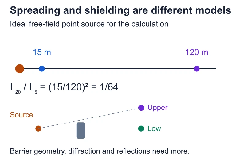$ For a free-field point source, intensity at 120 m is 1/64 of that at 15 m. A barrier can block a low receiver’s line of sight while leaving an upper receiver exposed; diffraction, reflection and source geometry also affect the sound received.

SECTION 8

Regulatory Frameworks & Connections to Broader Environmental Science

Noise pollution intersects with several other topics in the AP Environmental Science curriculum, including urbanization, biodiversity, public health, and environmental policy. Regulatory frameworks for noise differ markedly from those governing chemical pollutants because noise does not persist in the environment—once the source stops, the pollutant vanishes—yet the health effects of chronic exposure are cumulative and may be irreversible. This distinction shapes how policies are designed and enforced.

Dimension	Noise Pollution	Air Pollution (e.g., PM₂.₅)
Persistence	Ceases immediately when source stops; no residual contamination	Particulates can linger for hours to weeks; deposition creates secondary pollution
Health pathway	Stress hormones (cortisol), cardiovascular strain, hearing damage; effects are cumulative	Respiratory inflammation, carcinogenesis, cardiovascular damage; effects are cumulative
Measurement	Decibels (dB); A-weighted for human hearing (dBA); time-averaged metrics (Leq, Lden)	Micrograms per cubic meter (µg/m³); AQI indices
Major U.S. regulation	Noise Control Act (1972); largely defunded since 1982; regulation delegated to states/localities	Clean Air Act (1970, amended 1990); actively enforced by EPA with NAAQS
Environmental justice	Low-income communities near highways/airports disproportionately affected	Low-income communities near industrial zones disproportionately affected

Comparing noise pollution regulation with air pollution regulation

A critical point for the AP exam is that the EPA's Office of Noise Abatement and Control was effectively defunded in 1982, leaving the United States without a dedicated federal noise enforcement body. Today, noise regulation in the U.S. is a patchwork of state and local ordinances, whereas the European Union has pursued centralized strategic noise mapping under Directive 2002/49/EC. Looking ahead, growing research on the synergistic effects of noise and air pollution on cardiovascular disease, as well as acoustic ecology studies documenting the value of natural soundscapes for biodiversity, are pushing noise toward greater prominence in environmental policy. Students should also note the connection to environmental justice: communities of color and low-income populations are disproportionately located near highways, rail yards, and airports—the same areas with the highest noise exposures.

💡

AP Exam Connection

The APES exam may test noise pollution within the broader context of urbanization impacts or as part of a free-response question asking you to propose a solution to a community's combined air-and-noise exposure near a transportation corridor. Be prepared to describe both the health effects and the mitigation strategies, and to discuss environmental justice implications.

SECTION 9

Practice Problems

Question 1: CONCEPTUAL

A sound source produces a noise level of 80 dB. If a second identical source is placed next to the first and both operate simultaneously, the combined noise level will be closest to which of the following values?

A. 160 dB
B. 83 dB
C. 90 dB
D. 80 dB

Show answer (B)

Correct answer: B (83 dB). Because the decibel scale is logarithmic, combining two identical sources doubles the sound intensity, which corresponds to an increase of 10 × log₁₀(2) ≈ 3 dB—yielding about 83 dB. Option A (160 dB) incorrectly adds decibels arithmetically, which is never valid for a logarithmic scale. Option C (90 dB) would require a tenfold increase in intensity (ten identical sources). Option D (80 dB) ignores the second source entirely.

Question 2: BASIC CALCULATION

A factory emits noise at 100 dB measured at 10 m. Using the inverse square law and assuming open-air conditions with no reflections, what is the approximate sound level at 100 m from the factory?

A. 60 dB
B. 80 dB
C. 90 dB
D. 70 dB

Show answer (B)

Correct answer: B (80 dB). Distance increases by a factor of 10 (from 10 m to 100 m). By the inverse square law, intensity decreases by a factor of 10² = 100. In decibels: reduction = 10 × log₁₀(100) = 20 dB. So 100 − 20 = 80 dB. Option A (60 dB) overstates the reduction by applying a 40 dB drop, which would require a distance ratio of 100. Option C (90 dB) uses only a 10 dB reduction, corresponding to a factor-of-10 distance change rather than the squared relationship. Option D (70 dB) applies a 30 dB reduction, which corresponds to a factor-of-1000 decrease in intensity.

Question 3: INTERMEDIATE

A community group finds that traffic noise in their neighborhood averages 72 dB during the day. A proposed vegetation buffer of 40 m depth is expected to reduce noise by 5 dB. Which of the following statements best evaluates whether this mitigation is sufficient to meet the WHO daytime guideline of 55 dB?

A. The buffer is sufficient because 72 − 5 = 67 dB, which is below the 70 dB caution threshold.
B. The buffer is insufficient because 72 − 5 = 67 dB, which still exceeds the WHO guideline of 55 dB by 12 dB; additional strategies such as sound walls or source reduction would be needed.
C. The buffer is sufficient because vegetation absorbs noise exponentially, so the actual reduction will be much greater than 5 dB.
D. The buffer is insufficient because vegetation buffers only reduce perceived noise psychologically and provide no measurable dB reduction.

Show answer (B)

Correct answer: B. A 5 dB reduction brings the level to 67 dB, which still exceeds the WHO guideline (55 dB) by 12 dB—a substantial exceedance representing approximately 16 times the recommended intensity. Option A confuses the WHO 55 dB guideline with a generic 70 dB benchmark. Option C overstates the efficacy of vegetation; actual attenuation by vegetation is modest and roughly linear with dense buffer width, not exponential. Option D incorrectly denies any measurable acoustic benefit from vegetation; research documents 3–5 dB reductions for sufficiently dense, deep plantings.

Question 4: APPLIED

4 pts

A research team wants to determine whether chronic noise from a nearby highway (average 78 dB at the road edge) is affecting the breeding success of a ground-nesting bird species in an adjacent grassland. Design a field investigation to test this hypothesis. (a) State a testable hypothesis. (b) Describe an appropriate experimental design, including the independent variable, dependent variable, and at least one controlled variable. (c) Explain how sampling sites should be selected and how many replicates would be appropriate. (d) Identify one potential confounding variable and explain how the design accounts for it.

Show answer

Point-by-point rubric: (a) Hypothesis (1 point): Award 1 point for a clearly stated, testable hypothesis. Example: "Breeding success (measured as number of fledglings per nest) of the ground-nesting bird species decreases as ambient noise level increases with proximity to the highway." (b) Experimental design (1 point): Award 1 point for correctly identifying the independent variable (distance from highway or measured ambient noise level at each sampling site), the dependent variable (breeding success—e.g., number of fledglings per nest, hatching rate, or nest survival rate), and at least one controlled variable (e.g., habitat type, vegetation density, elevation, time of season when nests are monitored). The design should establish transects at varying distances from the highway (e.g., 50 m, 200 m, 500 m, 1000 m) with noise measurements taken at each distance. (c) Sampling design (1 point): Award 1 point for describing a systematic sampling approach with adequate replication. Sites should be selected along multiple parallel transects perpendicular to the highway to account for spatial variability. At least 3–5 replicates per distance category are recommended. Noise levels should be measured with calibrated sound level meters at each nest site during the breeding season. (d) Confounding variable (1 point): Award 1 point for identifying a plausible confounding variable (e.g., predation rates may differ with proximity to the road, road-edge effects on vegetation structure, visual disturbance from vehicles, chemical pollutants from traffic exhaust) and explaining how the design accounts for it (e.g., monitoring predation at all sites, ensuring habitat structure is comparable across distance categories, or including predator exclusion cages at a subset of nests to isolate noise effects from predation effects).

Question 5: CRITICAL THINKING

4 pts

A city monitors average daytime noise at four locations over a two-year period. The data are shown below: Location A (downtown): Year 1 = 74 dB, Year 2 = 71 dB (new electric bus fleet deployed) Location B (highway residential): Year 1 = 68 dB, Year 2 = 68 dB (no change) Location C (industrial zone): Year 1 = 82 dB, Year 2 = 78 dB (sound wall installed) Location D (park): Year 1 = 48 dB, Year 2 = 52 dB (new amphitheater opened) (a) Calculate the factor by which sound intensity decreased at Location A between Year 1 and Year 2. (b) Identify which location(s), if any, exceed the WHO daytime guideline of 55 dB in Year 2 and describe the health significance. (c) For Location D, explain why a 4 dB increase might concern environmental managers despite the absolute level still being relatively low. (d) Propose one additional data collection effort that would make this monitoring program more useful for policymakers.

Show answer

Point-by-point rubric: (a) Calculation (1 point): Award 1 point for correctly calculating the intensity ratio. The dB decrease is 74 − 71 = 3 dB. Using I₂/I₁ =

10^{Δβ/10}

10^{3/10}

10^{0.3}

≈ 2.0. Therefore, the sound intensity at Location A decreased by approximately a factor of 2 (i.e., intensity was halved). Accept values between 1.9 and 2.1. (b) WHO guideline comparison (1 point): Award 1 point for correctly identifying that Locations A (71 dB), B (68 dB), and C (78 dB) all exceed 55 dB in Year 2, while Location D (52 dB) does not. Health significance: chronic exposure to levels above 55 dB is associated with elevated cortisol levels, increased risk of hypertension and cardiovascular disease, sleep disruption, and reduced cognitive performance—particularly concerning for Location C, which remains 23 dB above the guideline. (c) Ecological/social significance of Location D's increase (1 point): Award 1 point for a substantive explanation. Although 52 dB is below the human health guideline, the park may serve as an acoustic refuge for wildlife that depend on low-noise environments for communication, foraging, and predator detection. A 4 dB increase represents a roughly 2.5-fold increase in sound intensity, which can mask bird songs and other animal vocalizations. Additionally, parks often represent the quietest accessible areas for residents seeking respite from urban noise, so degrading this acoustic environment reduces its recreational and mental-health value. (d) Additional data collection (1 point): Award 1 point for a reasonable, specific proposal. Examples include: measuring nighttime noise levels (which have stricter WHO guidelines of 40–45 dB), recording frequency-spectrum data to distinguish low-frequency traffic noise from other sources, conducting community health surveys to correlate noise exposure with self-reported outcomes, deploying continuous monitoring rather than snapshot measurements, or conducting biodiversity surveys at each location to assess ecological impacts.

SUMMARY

Summary

Noise pollution is unwanted or harmful sound produced by anthropogenic activities—principally transportation, industry, construction, and military operations. Sound intensity is measured on the logarithmic decibel (dB) scale, where every 10 dB increase represents a tenfold increase in intensity. The key formula β = 10 × log₁₀(I/I₀) relates intensity to the dB reading, and the inverse square law (I = P/4πr²) governs how sound attenuates with distance from a point source—doubling the distance reduces intensity by approximately 6 dB.

Human health effects include noise-induced hearing loss (NIHL) above 85 dB, cardiovascular stress, sleep disruption, and cognitive impairment from chronic exposure above the WHO guideline of 55 dB. Ecological effects include disrupted animal communication, altered species distributions, and marine mammal strandings linked to naval sonar. Mitigation strategies range from source controls (the most effective) and sound barriers to zoning and vegetation buffers. In the U.S., federal noise enforcement was largely abandoned after 1982, leaving regulation to states and localities—an important environmental justice concern given the disproportionate exposure of low-income and minority communities.