Island Biogeography - AP Environmental Science

SECTION 1

Historical Context & Motivation

For centuries, naturalists noticed a curious pattern: oceanic islands tend to harbor fewer species than comparable areas on the mainland, yet the species they do support are often found nowhere else on Earth. Charles Darwin's observations in the Galápagos and Alfred Russel Wallace's surveys of the Malay Archipelago laid the qualitative groundwork, but a predictive, quantitative framework did not emerge until the mid-twentieth century. The question that drove early biogeographers was deceptively simple—why do some islands have more species than others? Answering it required moving beyond species lists and toward the dynamic processes of colonization and extinction.

1835 • Darwin in the Galápagos

Charles Darwin collects finches and mockingbirds across the Galápagos Islands, noting that species composition varies by island size and distance from South America—observations that later shape his theory of natural selection.

1876 • Wallace's Biogeographic Regions

Alfred Russel Wallace publishes 'The Geographical Distribution of Animals,' establishing major biogeographic realms and identifying the importance of barriers—water gaps, mountain ranges—in shaping species distributions on islands.

1963 • MacArthur & Wilson's Theory

Robert MacArthur and E. O. Wilson publish a landmark paper proposing that species richness on an island reaches a dynamic equilibrium determined by immigration and extinction rates—the core of the Theory of Island Biogeography.

1967 • The Theory of Island Biogeography (book)

MacArthur and Wilson expand their model into a full monograph, introducing the species–area relationship and formalizing the effects of island size and distance on biodiversity. The book becomes one of the most cited works in ecology.

1969 • Simberloff & Wilson's Defaunation Experiment

Daniel Simberloff and E. O. Wilson fumigate small mangrove islands in the Florida Keys, eliminating all arthropods. Recolonization proceeds exactly as the equilibrium model predicts—closer, larger islands recover faster and with more species—providing the first rigorous experimental test.

The MacArthur–Wilson framework transformed ecology by treating species richness not as a fixed attribute of a place but as the outcome of two opposing processes—immigration and extinction—that continuously adjust toward an equilibrium number of species. This dynamic perspective also opened a powerful analogy: habitat fragments on the mainland can be modeled as 'islands' in a 'sea' of inhospitable land, an insight that now lies at the heart of modern conservation biology and the design of nature reserves.

SECTION 2

Core Principles & Definitions

The Theory of Island Biogeography rests on a small set of elegant ideas that, taken together, predict how many species an island will support at equilibrium. Understanding each principle individually is essential before exploring the mathematics and conservation applications that follow.

Immigration Rate

The rate at which new species colonize an island from a mainland source pool. Immigration declines as more species accumulate because fewer novel species remain to arrive.

Extinction Rate

The rate at which established species die out on the island. Extinction increases as more species are present because of greater competition, predation, and limited niche space.

Dynamic Equilibrium

Species richness stabilizes where the immigration curve intersects the extinction curve. The identity of species may turn over continuously even though the total number stays roughly constant.

Distance Effect

Islands farther from the mainland source have lower immigration rates—fewer propagules and individuals reach them—so their equilibrium species richness is lower.

Area Effect

Larger islands support more habitat diversity and larger populations, leading to lower extinction rates. They also present bigger 'targets' for colonizing species, slightly increasing immigration.

✦

KEY TAKEAWAY

Think of an island's species count like the water level in a bathtub with the faucet on and the drain open. Immigration is the faucet, extinction is the drain, and the equilibrium level depends on both flow rates. A large, close island has a wide-open faucet and a slow drain, so it fills high. A small, remote island has a trickle coming in and a fast drain, so its level stabilizes much lower. Even at equilibrium, water is always flowing in and out—just as species are always arriving and disappearing.

Two additional nuances are worth noting. First, the model treats the mainland as an effectively infinite source pool of species whose composition does not change. Second, species turnover at equilibrium means the set of species on the island is not static; the rate at which new species replace extinct ones is called the turnover rate, and it is highest on small, near islands where both immigration and extinction rates are elevated.

SECTION 3

The Equilibrium Model—Visualized

The most iconic diagram in island biogeography is the crossing of immigration and extinction curves. The graph below illustrates four scenarios by combining two levels of island size (large vs. small) with two levels of distance from the mainland (near vs. far). Where each immigration curve crosses each extinction curve, a distinct equilibrium species number (Ŝ) is predicted.

The dashed curves represent immigration rates for near (cyan) and far (violet) islands; they decline as species accumulate. Solid curves represent extinction rates for small (emerald) and large (pink) islands; they rise with species richness. The four intersection points (colored dots) indicate the predicted equilibrium species numbers (Ŝ). Note that Ŝ₁ (large, near) is the highest and Ŝ₄ (small, far) is the lowest.

Several features of this diagram deserve emphasis. First, the immigration curve is concave-up because as species accumulate, the probability that the next colonist represents a species already present increases, reducing the effective immigration of new species. Second, the extinction curve is concave-down because each additional species added to a crowded island faces disproportionately more competition for finite resources. Third, the turnover rate at equilibrium equals the y-value where the curves intersect: small, near islands have higher turnover than large, far islands even though the latter may support more total species.

A forested island, mainland and field observer accompany exact species-identity snapshots and illustrative crossing rate lines. Species richness can stay the same across two snapshots even though one species disappears and another arrives. A stable count can therefore accompany continuing turnover.

Equilibrium does not freeze the cast. Species richness can stay the same across two snapshots even though one species disappears and another arrives. A stable count can therefore accompany continuing turnover. 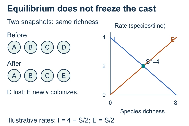Species richness can stay the same across two snapshots even though one species disappears and another arrives. A stable count can therefore accompany continuing turnover.

SECTION 4

Mathematical Framework

While the AP Environmental Science exam does not require you to derive the equilibrium model, a quantitative familiarity with the species–area relationship and the logic of equilibrium is expected. Two key equations underpin island biogeography.

SPECIES–AREA RELATIONSHIP

S = c × A^z

Where S = number of species, A = area of the island (km²), c = a taxon- and region-specific constant, and z = the slope of the species–area curve on a log–log plot (typically 0.20–0.35 for oceanic islands).

Taking the logarithm of both sides yields a linear relationship: log S = log c + z × log A. When you plot log(species) against log(area) for a group of islands, the data fall along a straight line with slope z and y-intercept log c. A higher z means species richness is more sensitive to area; isolated archipelagoes typically have steeper slopes than mainland habitat patches.

EQUILIBRIUM CONDITION

dS/dt = I(S) − E(S) = 0 at Ŝ

At equilibrium, the immigration rate I(S) equals the extinction rate E(S). Both are functions of the current number of species S. The equilibrium species richness Ŝ is the value of S where I(S) = E(S).

💡

AP EXAM TIP

The species–area equation S = cA^z is the quantitative relationship you are most likely to encounter on the APES exam. Be comfortable interpreting log–log graphs and predicting how a 50% reduction in habitat area affects species richness. Remember: because z is less than 1, halving the area does NOT halve the species count—it reduces it by roughly 15–25% depending on the z value.

SECTION 5

Habitat Fragments as Virtual Islands

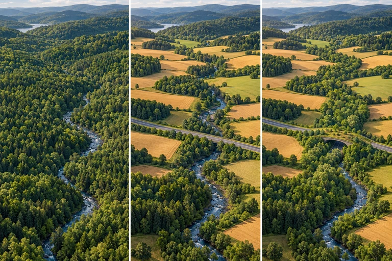
One of the most far-reaching applications of island biogeography is its extension to habitat fragmentation on the mainland. When a continuous forest is broken into patches by roads, agriculture, or urban development, each patch behaves like an island surrounded by an inhospitable 'sea' of altered landscape. The same principles apply: smaller patches lose species faster, and more isolated patches receive fewer immigrants. This analogy has guided the design of nature reserves and wildlife corridors for decades.

Reserve design guidelines derived from island biogeography. For each criterion (size, distance, corridors, shape), the left option supports higher species richness. A single large reserve outperforms several small ones (the famous SLOSS debate), nearby reserves exchange species more easily, corridors restore connectivity, and round reserves minimize edge effects.

The SLOSS debate (Single Large Or Several Small) has been one of conservation biology's longest-running discussions. MacArthur–Wilson theory originally favored a single large reserve because of lower extinction rates. However, ecologists such as Dan Simberloff pointed out that several small reserves can capture more habitat diversity and protect against catastrophic events—a wildfire that burns one reserve may leave others intact. Modern consensus recognizes that the optimal strategy depends on the landscape context, the target taxa, and the degree of connectivity among patches. Wildlife corridors—strips of habitat connecting fragments—can provide the benefits of both approaches by allowing gene flow and recolonization across a network of reserves.

SECTION 6

Worked Example: Predicting Species Loss from Habitat Reduction

A common AP-level application asks you to use the species–area relationship to estimate the effect of deforestation on species richness. Let's work through a representative problem step by step.

ℹ

PROBLEM

A tropical forest island originally covers 10,000 km² and supports approximately 500 bird species. Logging reduces the forested area to 1,000 km². Using a z-value of 0.30, estimate the number of bird species expected to remain after the habitat loss.

Species–Area Calculation

1
Step 1 — Identify Given Values

Original area A₁ = 10,000 km². Original species count S₁ = 500. Reduced area A₂ = 1,000 km². The z-value = 0.30.
2
Step 2 — Set Up the Ratio

Because S = cA^z, we can write S₂ / S₁ = (A₂ / A₁)^z. The constant c cancels out, which is extremely convenient because c is rarely known precisely.
3
Step 3 — Calculate the Area Ratio

A₂ / A₁ = 1,000 / 10,000 = 0.10. The area has been reduced to 10% of its original extent.

Area ratio = 0.10
4
Step 4 — Raise to the Power z

(A₂ / A₁)^z = 0.10^0.30. Using a calculator: 0.10^0.30 = 10^−0.30 ≈ 0.501.

Species ratio ≈ 0.501
5
Step 5 — Compute New Species Count

S₂ = S₁ × 0.501 = 500 × 0.501 ≈ 251 species.

≈ 251 bird species expected to survive
6
Step 6 — Interpret the Result

Reducing the habitat by 90% eliminates approximately 50% of bird species. This is the hallmark of the species–area curve: species loss is not proportional to area loss but follows a power-law function. Even so, the loss of roughly 249 species from a single island would be catastrophic for regional biodiversity.

SECTION 7

Strengths & Limitations of the Model

Like all models, the Theory of Island Biogeography simplifies complex ecological reality to generate testable predictions. Understanding both its power and its blind spots is essential for applying it correctly on the AP exam and in real-world conservation planning.

Strengths	Limitations
Provides a clear, quantitative prediction (Ŝ) testable with field data.	Treats all species as ecologically equivalent—ignores differences in dispersal ability, trophic level, and body size.
Successfully predicts broad patterns (species–area curves) across taxa and biomes.	Ignores speciation—important on large, ancient islands (e.g., Madagascar) where in-situ evolution adds species.
Applicable to mainland habitat fragments, guiding reserve design and corridor planning.	Assumes a homogeneous mainland source pool with constant composition—unrealistic for degraded mainland habitats.
Experimentally supported (Simberloff & Wilson mangrove island experiments; recolonization after volcanic eruptions).	Does not account for habitat heterogeneity within an island—a topographically complex island may support more species than a flat one of equal area.
Simple enough to be taught, applied, and communicated to policymakers.	Edge effects, matrix quality (the nature of the 'sea' around habitat islands), and disturbance regimes are not explicitly modeled.

Strengths and limitations of the MacArthur–Wilson equilibrium model

✦

KEY TAKEAWAY

The island biogeography model is like a GPS navigation app—remarkably useful for planning a route (reserve design), but it does not tell you about the potholes (edge effects), road closures (disturbance), or scenic detours (unique evolutionary history) you'll encounter along the way. Always use it as a first approximation and layer in local ecological knowledge.

SECTION 8

Connections to Modern Conservation Biology

Island biogeography does not exist in an intellectual vacuum—it connects directly to several advanced ecological concepts that appear across the APES curriculum and in current research. The table below maps each core idea from island biogeography to its broader conservation counterpart.

Island Biogeography Concept	Advanced Conservation Application
Species–area relationship (S = cA^z)	Predicting extinction debt — species that are doomed but haven't gone extinct yet after habitat loss.
Distance effect on immigration	Metapopulation theory — networks of subpopulations connected by dispersal; source–sink dynamics.
Area effect on extinction	Minimum viable population (MVP) analysis — below a critical area, populations become too small to avoid inbreeding depression and stochastic extinction.
Dynamic equilibrium / turnover	Landscape ecology — understanding how habitat mosaics, edge effects, and disturbance regimes influence biodiversity over time.
Reserve design (SLOSS, corridors)	Systematic conservation planning — tools like Marxan use species–area relationships and connectivity models to optimize reserve networks globally.

Island biogeography concepts mapped to modern conservation applications

Perhaps the most urgent contemporary application is the concept of extinction debt. When a habitat is reduced, the species–area relationship predicts a new, lower equilibrium. However, species do not vanish instantly; some persist for years or decades in populations too small to be viable in the long run. These 'living dead' species represent a debt that nature will eventually 'collect.' Recognizing extinction debt is critical because it means current species counts in recently fragmented habitats overestimate the long-term biodiversity those habitats can sustain, creating a false sense of security if used uncritically in conservation assessments.

Three qualitative forest landscapes show continuous woodland, fragmented woodland and a restored vegetated road crossing. Equal total reserve area can conceal differences in core habitat. With a one-unit edge zone, one 10-by-10 square retains 64 square units of core, while four 5-by-5 squares retain 36 in total.

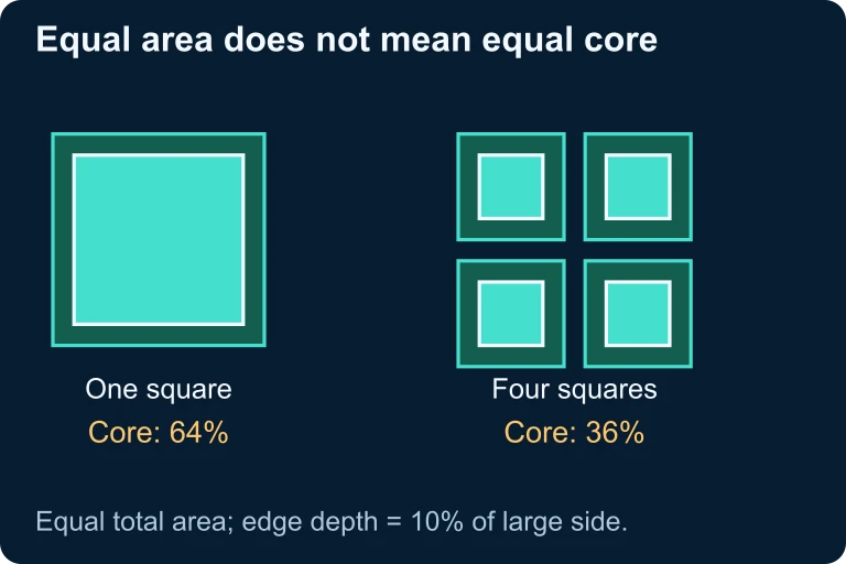Equal area does not mean equal core. With a one-unit edge depth, one 10-by-10 square contains 64 square units of core. Four 5-by-5 squares have the same total area but only 36 square units of core. With a one-unit edge depth, one 10-by-10 square contains 64 square units of core. Four 5-by-5 squares have the same total area but only 36 square units of core.

SECTION 9

Practice Problems

Question 1: CONCEPTUAL

According to the equilibrium model of island biogeography, which island would be expected to have the highest species richness at equilibrium?

A. A small island far from the mainland
B. A large island far from the mainland
C. A small island near the mainland
D. A large island near the mainland

Show answer (D)

D is correct. A large island near the mainland has the highest equilibrium species richness because it combines a high immigration rate (nearness to the source pool) with a low extinction rate (large area provides more habitat niches and supports larger, more resilient populations). Choice A is the worst combination (low immigration, high extinction). Choice B has lower immigration due to distance even though its large size reduces extinction. Choice C benefits from proximity but its small size drives higher extinction rates.

Question 2: BASIC CALCULATION

An island of 5,000 km² supports 200 amphibian species. Using the species–area relationship (S = cA^z) and z = 0.25, approximately how many amphibian species would be expected on a nearby island of 500 km² with the same source pool?

A. 20 species
B. 112 species
C. 150 species
D. 178 species

Show answer (B)

B is correct. S₂/S₁ =

(A₂/A₁)^z

(500/5,000)^{0.25}

(0.1)^{0.25}

. Using the rule that

0.1^{0.25}

10^{−0.25}

≈ 0.562, we get S₂ = 200 × 0.562 ≈ 112 species. Choice A (20) incorrectly treats the relationship as directly proportional (dividing by 10). Choice C (150) underestimates the effect of area reduction. Choice D (178) results from using too low a z-value (roughly z = 0.10).

Question 3: INTERMEDIATE

A conservation biologist observes that a recently fragmented forest patch of 100 km² still contains 90% of the species found before fragmentation, even though the species–area relationship predicts only 70% should persist at equilibrium. Which concept best explains this discrepancy?

A. The z-value for this region must be higher than assumed
B. Extinction debt—species committed to extinction have not yet disappeared
C. Edge effects have increased habitat diversity
D. Immigration from the surrounding matrix has added new species

Show answer (B)

B is correct. Extinction debt describes the time lag between habitat loss and the eventual disappearance of species whose populations are no longer viable. The 90% figure is temporarily inflated and will decline toward the predicted 70% over time. Choice A is incorrect because a higher z-value would predict even fewer species at equilibrium, making the discrepancy larger, not smaller. Choice C is incorrect because edge effects generally reduce interior habitat quality and harm interior specialists. Choice D is unlikely because the surrounding matrix in a fragmented landscape is typically hostile (farmland, urban), not a species source.

Question 4: APPLIED

4 pts

A team of ecologists wants to test whether wildlife corridors increase the species richness of small mammal communities in fragmented agricultural landscapes. Design an investigation to test this hypothesis. (a) State a testable hypothesis. (1 point) (b) Describe the experimental design, including treatment and control groups, and identify at least two variables that should be held constant. (2 points) (c) Describe the type of data to be collected and explain how the results would either support or refute the hypothesis. (1 point)

Show answer

(a) 1 point — Hypothesis: Forest fragments connected by wildlife corridors will have significantly higher small mammal species richness than fragments of equal size that are not connected by corridors. (b) 2 points (1 for design with treatment/control, 1 for controlled variables) — Select at least 10 pairs of forest fragments matched for area (e.g., 5 ha each), distance from the nearest large source forest, and surrounding land use. Within each pair, randomly assign one fragment to receive a planted corridor (at least 50 m wide and 200 m long) connecting it to a larger source forest, while the other fragment serves as an unconnected control. Controlled variables include fragment area, surrounding matrix type, and the study duration. Each fragment should be sampled simultaneously over a minimum of two years to account for seasonal variation. (c) 1 point — Collect data on the number of small mammal species detected in each fragment using standardized live-trapping (Sherman traps in a grid, checked for 5 consecutive nights per season). Compare mean species richness between corridor-connected and control fragments using a paired t-test or equivalent. If corridor-connected fragments have significantly higher species richness (p < 0.05), the hypothesis is supported, indicating corridors enhance immigration. If there is no significant difference, the hypothesis is refuted.

Question 5: CRITICAL THINKING

4 pts

The following data were collected for reptile species on six islands in a tropical archipelago. Island A: Area = 10,000 km², Species = 150 Island B: Area = 5,000 km², Species = 120 Island C: Area = 1,000 km², Species = 75 Island D: Area = 500 km², Species = 60 Island E: Area = 100 km², Species = 35 Island F: Area = 10 km², Species = 15 (a) Using the species–area relationship S =

cA^z

, calculate z using islands A and F. Show your work. (2 points) (b) Island C is 20 km from the mainland while Island D is 350 km away. Despite being half the area of Island C, Island D has nearly as many species. Propose a biological explanation for why distance from the mainland alone does not fully explain this observation. (1 point) (c) A proposed development would reduce Island B's forested area from 5,000 km² to 2,500 km². Using the z-value you calculated in (a), predict the number of reptile species that would remain. Discuss one limitation of using this prediction for conservation policy. (1 point)

Show answer

(a) 2 points (1 for setup, 1 for correct calculation) — Using S =

cA^z

for Islands A and F: 150 = c × 10,

000^z

and 15 = c ×

10^z

. Dividing: 150/15 =

(10,000/10)^z

→ 10 = 1,

000^z

→ log(10) = z × log(1,000) → 1 = z × 3 → z = 0.333 (or approximately 0.33). (b) 1 point — Island D may have greater habitat heterogeneity than its area alone suggests—for example, elevational gradients, multiple vegetation types, or unique microhabitats like caves and rocky outcrops that support specialized reptile species. Additionally, ocean currents or stepping-stone islets between Island D and the mainland may facilitate dispersal despite the greater distance, effectively reducing functional isolation. (c) 1 point — S₂ = S₁ ×

(A₂/A₁)^z

= 120 ×

(2,500/5,000)^{0.333}

= 120 ×

(0.5)^{0.333}

. Calculating:

(0.5)^{0.333}

2^{−0.333}

≈ 0.794. S₂ = 120 × 0.794 ≈ 95 species. Approximately 25 species (≈21%) would be lost. A key limitation is that the species–area relationship does not specify which species will be lost; if the development disproportionately destroys the habitat of rare endemic species, the conservation impact could be far more severe than the raw number suggests. The model also assumes that all habitats are equally likely to be lost, which is rarely the case in real development scenarios.

SUMMARY

Summary

The Theory of Island Biogeography, developed by MacArthur and Wilson in the 1960s, predicts that an island's species richness reaches a dynamic equilibrium where the immigration rate of new species equals the extinction rate of established species. Two key factors determine the equilibrium number: the distance effect (farther islands receive fewer colonists) and the area effect (larger islands have lower extinction). The quantitative backbone of the theory is the species–area relationship (S = cA^z), which enables predictions of species loss following habitat reduction.

Beyond oceanic islands, this framework applies to any insular habitat—habitat fragments, mountaintops, lakes, and nature reserves—making it central to conservation biology. Key design principles favor reserves that are large, close together, connected by corridors, and round in shape. The concept of extinction debt warns that present species counts may overestimate the long-term viability of fragmented landscapes. For the AP exam, be prepared to interpret species–area graphs, perform calculations with S = cA^z, explain the SLOSS debate, and connect island biogeography to real-world conservation scenarios involving species turnover and habitat fragmentation.