Eutrophication - AP Environmental Science

SECTION 1

Historical Context & Motivation

For most of human history, lakes, rivers, and coastal waters cycled nutrients slowly enough that primary producers and decomposers remained in dynamic equilibrium. The industrialization of agriculture in the mid-twentieth century, however, introduced unprecedented quantities of nitrogen (N) and phosphorus (P) into waterways through synthetic fertilizers, concentrated animal feeding operations, and municipal wastewater. Scientists began documenting widespread algal blooms and oxygen-depleted zones that devastated fisheries, tourism economies, and drinking-water supplies. Understanding eutrophication—the process by which excess nutrient loading accelerates biological productivity to the point of ecological collapse—became one of the defining challenges of modern environmental science.

1940s • The Green Revolution Begins

The Haber–Bosch process enables mass production of synthetic nitrogen fertilizers, dramatically increasing reactive nitrogen inputs to watersheds across North America and Europe.

1960s • Lake Erie "Dies"

Massive algal blooms and fish kills in Lake Erie draw national attention. Phosphorus from detergents and sewage is identified as the primary culprit, catalyzing the modern eutrophication research agenda.

1972 • U.S. Clean Water Act

Federal legislation mandates point-source nutrient controls and establishes the National Pollutant Discharge Elimination System (NPDES), reducing direct sewage phosphorus inputs to many waterways.

1985 • Gulf of Mexico Dead Zone Mapped

Researchers document a seasonal hypoxic zone exceeding 10,000 km² at the Mississippi River delta, linking it to agricultural nitrogen runoff from the Corn Belt—a textbook case of cultural eutrophication.

2014 • Toledo Water Crisis

A toxic Microcystis bloom in Lake Erie contaminates Toledo, Ohio's drinking water with microcystin, forcing a two-day "do-not-drink" advisory for 500,000 residents and renewing urgency around phosphorus reduction.

These milestones raise a central question for environmental scientists: How do excess nutrients transform aquatic ecosystems, and what strategies can reverse or prevent this transformation? The sections that follow develop the ecological mechanisms, quantitative tools, and policy frameworks you need to answer that question on the AP exam and beyond.

SECTION 2

Core Principles & Definitions

Eutrophication sits at the intersection of nutrient cycling, aquatic ecology, and pollution science. Before examining specific mechanisms, it is essential to distinguish two related but distinct processes. Natural eutrophication is the slow, geological-timescale enrichment of a water body as sediments and organic matter accumulate over millennia—essentially the aging of a lake. Cultural (anthropogenic) eutrophication is the same trajectory compressed into years or decades by human nutrient inputs. The AP exam almost exclusively tests the cultural form.

Limiting Nutrients

Phosphorus is typically the limiting nutrient in freshwater systems, while nitrogen limits productivity in most marine and estuarine environments. Identifying the correct limiting nutrient is critical for targeted remediation.

Algal Bloom Formation

When the limiting nutrient becomes abundant, phytoplankton and cyanobacteria reproduce exponentially, forming dense surface mats (blooms) that block sunlight from reaching submerged aquatic vegetation.

Decomposition & Oxygen Demand

When algae die, aerobic bacteria decompose the biomass, consuming dissolved oxygen (DO) at rates that outpace atmospheric re-aeration. This process creates biochemical oxygen demand (BOD).

Hypoxia & Dead Zones

When DO drops below approximately 2 mg/L, a condition called hypoxia, most fish and invertebrates cannot survive. Persistent hypoxic areas are termed "dead zones." Over 500 coastal dead zones have been documented globally.

Positive Feedback Loops

Anoxic sediments release stored phosphorus back into the water column (internal loading), which fuels additional blooms even after external inputs are reduced—a feedback mechanism that complicates restoration efforts.

✦

KEY TAKEAWAY

Think of a lake like a self-cleaning aquarium. Under normal conditions, the biological filter (decomposers, plants, and sediments) processes waste at the rate it arrives. Cultural eutrophication is analogous to massively overfeeding the aquarium—the filter cannot keep pace, algae coat the glass, oxygen plummets, and fish die. Restoring equilibrium requires reducing the feed rate (nutrient inputs) and sometimes cleaning out accumulated debris (internal nutrient loading).

SECTION 3

Visual Explanation — The Eutrophication Cascade

The upper panel traces the four-stage cascade from nutrient input to hypoxia. The lower cross-section shows a eutrophic lake with a dense algal mat blocking sunlight, aerobic decomposers consuming dissolved oxygen at depth, and anoxic sediments releasing stored phosphorus—a positive feedback loop that sustains eutrophic conditions even after external loading is reduced.

The diagram above illustrates the self-reinforcing nature of eutrophication. Notice that stage 4 (hypoxia) circles back into the system via internal phosphorus loading from anoxic sediments. Under aerobic conditions, iron-phosphorus complexes in sediment bind phosphate tightly. When bottom waters become anoxic, these complexes dissolve and release phosphate back into the water column, fueling additional algal blooms. This feedback mechanism explains why many eutrophic lakes remain impaired for years after external nutrient reductions—a phenomenon known as hysteresis in ecological restoration.

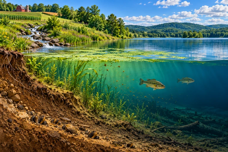A farm stream enters a cutaway lake with a partial green surface bloom, settling brown flecks, living fish in upper water and mussels near the bottom. Nutrient enrichment can increase algal production. Aerobic decomposition of sinking organic matter consumes dissolved oxygen, while mixing can replenish it. Hypoxia develops when oxygen demand exceeds replenishment.

Eutrophication oxygen mechanism. Nutrient enrichment can increase algal production. Aerobic decomposition of sinking organic matter consumes dissolved oxygen, while mixing can replenish it. Hypoxia develops when oxygen demand exceeds replenishment. 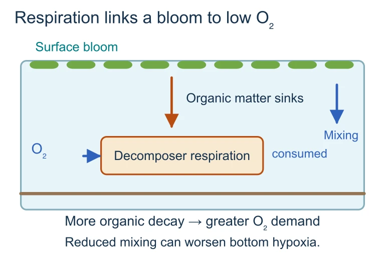Nutrient enrichment can increase algal production. Aerobic decomposition of sinking organic matter consumes dissolved oxygen, while mixing can replenish it. Hypoxia develops when oxygen demand exceeds replenishment.

SECTION 4

Mechanism — Nutrient Loading & Oxygen Dynamics

Although eutrophication is fundamentally an ecological process, several quantitative relationships appear on the AP Environmental Science exam and provide useful diagnostic tools. The three most relevant are: the relationship between nutrient loading and algal biomass, the biochemical oxygen demand (BOD) concept, and the dissolved oxygen (DO) sag curve.

LIEBIG'S LAW — LIMITING NUTRIENT

Growth Rate = f(min{[N], [P], [light], ...})

Primary productivity is controlled by whichever essential resource is in shortest supply relative to demand. In freshwater, phosphorus (P) is typically limiting because it has no significant gaseous phase and enters water mainly through weathering and runoff. In marine systems, nitrogen (N) is usually limiting because denitrification removes bioavailable N.

BIOCHEMICAL OXYGEN DEMAND (BOD)

BOD₅ = DO_initial − DO_final (measured over 5 days at 20 °C)

BOD₅ quantifies the mass of dissolved oxygen consumed by microorganisms decomposing organic matter in a sealed sample over five days at 20 °C. A pristine stream may have BOD₅ < 2 mg/L, whereas raw sewage can exceed 300 mg/L. Higher BOD signals greater organic pollution and eutrophic potential.

DISSOLVED OXYGEN SAG CURVE (STREETER–PHELPS)

D(t) = [k₁ × L₀ / (k₂ − k₁)] × (e^(−k₁t) − e^(−k₂t)) + D₀ × e^(−k₂t)

D(t) = oxygen deficit at time t; k₁ = deoxygenation rate constant; k₂ = reaeration rate constant; L₀ = initial BOD; D₀ = initial oxygen deficit. The curve dips to a critical point downstream of a pollution source where oxygen depletion is greatest, then recovers as reaeration exceeds consumption. In eutrophic waters, high L₀ values deepen and extend this sag.

💡

AP Exam Tip

You will not need to derive the Streeter–Phelps equation, but you should be able to interpret a DO sag curve, identify the zone of maximum oxygen deficit, and explain why the curve eventually recovers (reaeration rate exceeds decomposition rate as organic load diminishes downstream).

SECTION 5

Nutrient Sources — Point vs. Nonpoint

Effective eutrophication management requires distinguishing between point sources—discrete, identifiable discharge locations such as sewage outfalls and factory drains—and nonpoint sources (NPS), which represent diffuse inputs carried by overland flow, infiltration, and atmospheric deposition across broad landscapes. Since the Clean Water Act largely addressed point sources in the 1970s, nonpoint agricultural runoff has become the dominant contributor to cultural eutrophication in the United States.

Point sources (left, red) are regulated under the Clean Water Act's NPDES permit system, but they contribute only about 20% of the total nutrient load to U.S. waterways. Nonpoint sources (right, amber), primarily agricultural runoff, account for roughly 80% and are far more difficult to regulate because they are diffuse and episodic.

This distinction carries enormous policy implications. While point-source controls have achieved remarkable success since the 1970s—reducing phosphorus discharge from wastewater treatment plants by over 50% in many regions—nonpoint-source reductions depend on voluntary adoption of best management practices (BMPs) by millions of individual landowners. Common BMPs include riparian buffer strips, cover cropping, no-till agriculture, precision fertilizer application, and constructed wetlands that intercept nutrient-laden runoff before it reaches surface water. On the AP exam, expect to identify specific BMPs and explain why nonpoint-source pollution remains the dominant eutrophication driver despite decades of Clean Water Act enforcement.

SECTION 6

Worked Example — Phosphorus Loading & BOD Calculation

A municipal wastewater treatment plant discharges treated effluent into a small lake. Use the data below to estimate the annual phosphorus load and evaluate the lake's eutrophic status.

Annual Phosphorus Loading to a Lake

1
Step 1 — Identify Given Values

Effluent discharge rate: Q = 5.0 × 10⁶ L/day. Effluent total phosphorus concentration: C_P = 1.5 mg/L. Lake surface area: A = 2.0 km². We need the annual P load in kg/yr and the areal loading rate in g P/m²/yr.
2
Step 2 — Calculate Daily Phosphorus Load

Daily load = Q × C_P = (5.0 × 10⁶ L/day)(1.5 mg/L) = 7.5 × 10⁶ mg/day = 7.5 kg/day.

Daily P load = 7.5 kg/day
3
Step 3 — Convert to Annual Load

Annual load = 7.5 kg/day × 365 days/yr = 2,737.5 kg P/yr ≈ 2,738 kg P/yr.

Annual P load ≈ 2,738 kg/yr
4
Step 4 — Calculate Areal Loading Rate

Convert lake area: 2.0 km² = 2.0 × 10⁶ m². Convert annual load to grams: 2,738 kg × 1,000 g/kg = 2,738,000 g. Areal loading = 2,738,000 g ÷ 2.0 × 10⁶ m² = 1.37 g P/m²/yr.

Areal loading rate = 1.37 g P/m²/yr
5
Step 5 — Interpret the Result

The Vollenweider model classifies lakes with areal P loading above approximately 0.3–0.5 g P/m²/yr as eutrophic. At 1.37 g P/m²/yr, this lake exceeds the eutrophic threshold by a factor of roughly 3–4, indicating it is at high risk for persistent algal blooms and hypoxic conditions. Reducing the effluent phosphorus concentration to below 0.5 mg/L (tertiary treatment) would cut the load to approximately 0.46 g P/m²/yr, bringing the lake closer to the mesotrophic–eutrophic boundary.

Lake is well above the eutrophic threshold — intervention needed

SECTION 7

Remediation Strategies — Strengths & Limitations

Addressing eutrophication requires a portfolio of strategies operating at different scales—from farm-level nutrient management to basin-wide policy instruments. No single approach is sufficient, and each carries trade-offs between cost, effectiveness, and implementation speed.

Strategy	Strengths	Limitations
Tertiary wastewater treatment	Removes >95% of P from effluent; directly enforceable via NPDES permits	Expensive capital and operating costs; addresses only point sources (~20% of load)
Riparian buffer zones	Intercepts 50–85% of N and P in surface runoff; provides habitat, bank stabilization	Requires voluntary landowner participation; effectiveness varies with width, vegetation, and slope
Constructed wetlands	Low energy cost; removes N via denitrification and P via sedimentation; co-benefits for wildlife	Large land footprint; performance declines in cold climates; periodic harvesting of biomass required
Cover crops / no-till farming	Reduces erosion and nutrient runoff 30–60%; improves soil health; sequesters carbon	Requires farmer adoption and training; may slightly reduce yields in transition years; economic incentives needed
Alum / clay application (in-lake)	Binds dissolved P in sediment; rapid results; can break internal loading cycle	Treats symptom, not cause; repeated applications may be needed; potential aluminum toxicity at low pH

Comparison of common eutrophication remediation strategies

✦

KEY TAKEAWAY

In engineering, the most effective pollution control follows the principle of source reduction over end-of-pipe treatment. The same logic applies to eutrophication: it is far more cost-effective and ecologically sound to prevent nutrients from entering a waterway (via precision agriculture, buffer strips, and wetlands) than to remediate a lake after hypoxia has set in. In-lake treatments like alum are analogous to taking medication for chronic disease symptoms while continuing the lifestyle that caused the disease.

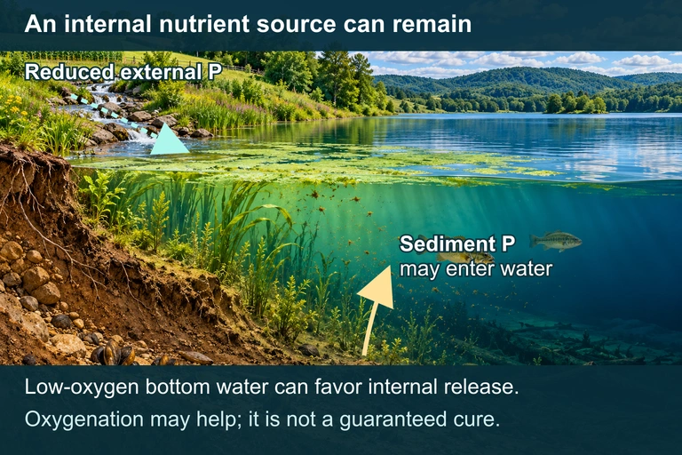A split-level lake scene shows a rooted shore, farmland stream and dark sediment bed. The companion distinguishes reduced external phosphorus input from conditional sediment release under low-oxygen bottom conditions. Reducing external phosphorus inputs can leave a conditional internal source in lake sediments. Oxygen conditions and management influence that pathway.

SECTION 8

Global Dead Zones & Climate Connections

Eutrophication is not merely a local water-quality issue—it intersects with several planetary-scale environmental challenges. The Gulf of Mexico dead zone, which averaged roughly 14,000 km² in recent years, is one of over 500 documented coastal hypoxic zones worldwide. Climate change exacerbates eutrophication through multiple pathways: warmer water holds less dissolved oxygen, stronger stratification inhibits mixing and reoxygenation, and more intense precipitation events flush larger nutrient pulses into waterways. Meanwhile, nutrient-enriched wetlands and estuaries produce nitrous oxide (N₂O), a potent greenhouse gas, creating a feedback between water pollution and atmospheric warming.

Feature	Eutrophication (this lesson)	Ocean Acidification (advanced)
Primary driver	Excess N and P from agriculture, sewage	Excess CO₂ absorbed by seawater
Affected parameter	Dissolved oxygen (DO)	pH and carbonate chemistry
Scale	Freshwater and coastal; local to regional	Global ocean
Key organisms affected	Fish, benthic invertebrates, submerged vegetation	Corals, mollusks, calcifying plankton
Interaction	Decomposition of algal blooms produces CO₂, lowering local pH	Lower pH may favor some harmful algal species, compounding eutrophication

Eutrophication vs. Ocean Acidification — conceptual comparison

The table above highlights how eutrophication connects to broader biogeochemical disruptions. On the AP exam, you may encounter questions linking eutrophication with climate change, the nitrogen cycle, or harmful algal blooms (HABs) that produce toxins such as microcystin and domoic acid. Recognizing these cross-topic connections will strengthen your ability to answer multi-concept free-response questions.

SECTION 9

Practice Problems

Question 1: CONCEPTUAL

A researcher studying a freshwater lake finds that adding phosphorus to water samples dramatically increases algal growth, while adding nitrogen produces no significant change. Which of the following conclusions is best supported by these results?

A. Nitrogen is the limiting nutrient in this lake.
B. Phosphorus is the limiting nutrient in this lake.
C. The lake is nitrogen-saturated and phosphorus-depleted, indicating an oligotrophic state.
D. Both nitrogen and phosphorus must be reduced simultaneously to control algal blooms.

Show answer (B)

B is correct. According to Liebig's Law of the Minimum, the nutrient in shortest supply relative to biological demand controls growth. Because only phosphorus addition stimulated algal growth, phosphorus is the limiting nutrient—the classic finding for freshwater systems. A is incorrect because adding nitrogen had no effect, meaning it is already sufficient. C is incorrect because being phosphorus-limited says nothing about trophic state; even eutrophic lakes can be P-limited. D is incorrect because the experimental data show that controlling phosphorus alone would reduce algal productivity.

Question 2: BASIC CALCULATION

A wastewater treatment plant discharges 8.0 × 10⁶ L/day of effluent containing 2.0 mg/L of total phosphorus into a stream. What is the daily phosphorus load in kilograms?

A. 1.6 kg/day
B. 16 kg/day
C. 160 kg/day
D. 1,600 kg/day

Show answer (B)

B is correct. Daily load = flow × concentration = (8.0 × 10⁶ L/day)(2.0 mg/L) = 16.0 × 10⁶ mg/day. Converting: 16.0 × 10⁶ mg × (1 g/1,000 mg) × (1 kg/1,000 g) = 16.0 kg/day. A (1.6 kg) results from an extra factor-of-ten conversion error. C (160 kg) and D (1,600 kg) result from failing to convert mg to kg correctly, omitting one or both division-by-1,000 steps.

Question 3: INTERMEDIATE

A lake has experienced cultural eutrophication. After ten years of strict external phosphorus reduction, water quality has not improved. Which mechanism most likely explains the continued eutrophic conditions?

A. Atmospheric nitrogen deposition from nearby power plants has replaced phosphorus as the growth-limiting nutrient.
B. Invasive fish species are consuming so much zooplankton that grazing pressure on algae has collapsed.
C. Anoxic bottom sediments are releasing previously stored phosphorus back into the water column, sustaining algal blooms via internal loading.
D. Climate change has increased water temperatures enough to permanently suppress dissolved oxygen regardless of nutrient levels.

Show answer (C)

C is correct. Internal phosphorus loading is the classic mechanism of hysteresis in eutrophic lakes. Under anoxic conditions, iron-bound phosphorus in sediments is released into the water column, sustaining algal blooms independently of external inputs. A is plausible in marine systems but does not explain continued eutrophication in a freshwater lake where P remains the limiting nutrient. B describes a trophic cascade that could worsen blooms but is not the most likely explanation when decades of P have accumulated in sediments. D overstates the role of temperature alone—warming reduces DO saturation by only a few mg/L and would not maintain full eutrophic conditions without continued nutrient supply.

Question 4: APPLIED

4 pts

A state environmental agency suspects that agricultural runoff from corn and soybean farms is causing eutrophication in a 50-hectare reservoir used for drinking water. Design a controlled investigation to determine whether phosphorus from agricultural runoff is the primary driver of algal blooms in the reservoir. In your response, include: (a) a testable hypothesis, (b) a description of the experimental setup including controls and variables, (c) the data you would collect and how, and (d) an explanation of how results would support or refute your hypothesis.

Show answer

Point 1 — Testable Hypothesis (1 pt): If phosphorus from agricultural runoff is the primary driver of algal blooms, then water samples receiving phosphorus additions will show significantly greater chlorophyll-a concentrations (a proxy for algal biomass) than samples receiving nitrogen additions or no additions. Point 2 — Experimental Setup (1 pt): Collect reservoir water in multiple identical clear containers (e.g., 20-L carboys). Establish at least four treatment groups with replicates (minimum 3 per group): (1) Control — no nutrient addition; (2) Phosphorus only — add KH₂PO₄ to raise [P] by 0.1 mg/L; (3) Nitrogen only — add KNO₃ to raise [N] by 1.0 mg/L; (4) Phosphorus + Nitrogen — both additions. All containers placed under identical light and temperature conditions. The independent variable is the type of nutrient added; the dependent variable is chlorophyll-a concentration; controlled variables include light, temperature, initial water source, and container volume. Point 3 — Data Collection (1 pt): Measure chlorophyll-a concentration (via fluorometry or spectrophotometry) and dissolved oxygen every 48 hours for 14 days. Also measure turbidity and cell counts of dominant algal species. Simultaneously, collect water samples from agricultural drainage ditches entering the reservoir and analyze them for total phosphorus and total nitrogen to confirm the composition of the runoff. Point 4 — Interpretation (1 pt): If the phosphorus-only and phosphorus + nitrogen treatments show significantly higher chlorophyll-a than the control and nitrogen-only treatments (assessed via statistical test such as ANOVA, p < 0.05), the hypothesis is supported—phosphorus is the limiting nutrient and agricultural P inputs are the primary eutrophication driver. If nitrogen-only treatments show equivalent or greater responses, the hypothesis is refuted, and nitrogen may be the limiting or co-limiting nutrient.

Question 5: CRITICAL THINKING

4 pts

The table below shows water quality data for three sampling stations along a river downstream of a city's wastewater outfall. Station A (0 km below outfall): DO = 8.5 mg/L, BOD₅ = 3 mg/L, Total P = 0.08 mg/L Station B (15 km below outfall): DO = 3.2 mg/L, BOD₅ = 18 mg/L, Total P = 0.45 mg/L Station C (45 km below outfall): DO = 7.0 mg/L, BOD₅ = 5 mg/L, Total P = 0.15 mg/L (a) Describe the pattern in dissolved oxygen from Station A to Station C and explain the biological processes responsible. (b) Identify which station is closest to the critical point on a DO sag curve and justify your reasoning. (c) Propose one structural and one regulatory strategy the city could implement to reduce eutrophication risk downstream and explain the mechanism by which each would help. (d) Explain why Station C shows higher DO than Station B, even though both are downstream of the outfall.

Show answer

Point 1 — Pattern Description (1 pt): Dissolved oxygen decreases from 8.5 mg/L at Station A (upstream or at the outfall, before significant decomposition has occurred) to 3.2 mg/L at Station B (15 km downstream) and then recovers to 7.0 mg/L at Station C (45 km downstream). This pattern is explained by the DO sag curve: at Station B, aerobic decomposition of the wastewater's organic matter (high BOD₅ = 18 mg/L) consumes dissolved oxygen faster than atmospheric reaeration can replenish it, causing the DO minimum. By Station C, most of the biodegradable organic matter has been consumed (BOD₅ drops to 5 mg/L), so reaeration from the atmosphere and photosynthesis exceed decomposition, and DO recovers. Point 2 — Critical Point Identification (1 pt): Station B (15 km downstream) is closest to the critical point because it has the lowest DO (3.2 mg/L) and the highest BOD₅ (18 mg/L). The critical point is defined as the location where the oxygen deficit is greatest—i.e., where the rate of oxygen consumption by decomposers equals the rate of reaeration, and DO reaches its minimum before recovery begins. Point 3 — Proposed Strategies (1 pt): Structural strategy: Upgrade the wastewater treatment plant to tertiary treatment (biological nutrient removal), which uses specialized bacteria to convert NH₄⁺ to N₂ gas (nitrification-denitrification) and chemical precipitation (e.g., alum or ferric chloride) to remove phosphorus. This directly reduces the nutrient and organic load entering the river, lowering both BOD and total P in the effluent. Regulatory strategy: Establish a Total Maximum Daily Load (TMDL) for phosphorus in the river, setting legally enforceable limits on the mass of P the wastewater plant and other sources can discharge per day, requiring the municipality to meet nutrient reduction targets on a defined timeline. Point 4 — Recovery Explanation (1 pt): Station C shows higher DO than Station B because by 45 km downstream, the majority of the labile organic matter introduced by the wastewater has already been decomposed. With less organic substrate available, microbial oxygen demand drops sharply (BOD₅ = 5 mg/L vs. 18 at Station B). Simultaneously, atmospheric oxygen continues to diffuse into the water across the air-water interface (reaeration), and photosynthesis by surviving aquatic plants and algae adds oxygen. Because the reaeration rate now exceeds the deoxygenation rate, dissolved oxygen recovers toward its saturation value—the ascending (recovery) limb of the Streeter-Phelps DO sag curve.

SUMMARY

Eutrophication — Summary Review

Summary

Eutrophication is the process by which excess nitrogen and phosphorus accelerate primary productivity in aquatic systems, triggering algal blooms that block sunlight, die, and decompose. The aerobic decomposition creates massive biochemical oxygen demand (BOD), driving dissolved oxygen below the hypoxic threshold of ~2 mg/L and creating dead zones. Phosphorus is typically the limiting nutrient in freshwater, while nitrogen limits marine systems. A critical positive feedback loop operates through internal phosphorus loading: anoxic sediments release stored P, fueling additional blooms even after external inputs are curtailed.

Remediation requires addressing both point sources (via tertiary wastewater treatment and NPDES permits) and nonpoint sources (via best management practices such as riparian buffers, cover crops, no-till farming, and constructed wetlands). Nonpoint agricultural runoff accounts for approximately 80% of nutrient loading in the U.S. and remains the greatest challenge. For the AP exam, remember the four-stage cascade (nutrient input → algal bloom → die-off → hypoxia), be prepared to interpret a dissolved oxygen sag curve, and understand why source reduction is more effective than in-lake remediation.