Dose Response Curve - AP Environmental Science

SECTION 1

Historical Context & Motivation

The idea that the severity of a poison's effect depends on how much of it enters the body seems intuitive today, but it took centuries to formalize this relationship into a quantitative science. The dose-response curve is the graphical representation of the relationship between the amount of a substance an organism is exposed to and the magnitude of the biological effect it produces. This concept lies at the heart of toxicology, environmental regulation, and risk assessment, enabling scientists to determine safe exposure thresholds and identify hazardous pollutant concentrations in air, water, and soil.

1538 • Paracelsus — "The Dose Makes the Poison"

Swiss physician Paracelsus articulated the foundational principle that all substances are potentially toxic — only the dose determines whether a substance acts as a remedy or a poison. This axiom remains the cornerstone of modern toxicology.

1927 • Trevan Introduces LD₅₀

British pharmacologist J.W. Trevan proposed the lethal dose 50 (LD₅₀) — the dose that kills 50% of a test population — as a standardized metric for comparing the acute toxicity of different substances.

1954 • Probit Analysis and Dose-Response Modeling

D.J. Finney's textbook on probit analysis gave scientists a rigorous statistical framework for fitting dose-response data to sigmoid curves, enabling quantitative estimation of thresholds such as LD₅₀ and EC₅₀.

1970s • EPA and Regulatory Toxicology

The creation of the U.S. Environmental Protection Agency catalyzed the systematic use of dose-response data in setting legally enforceable pollutant standards for drinking water, air quality, and pesticide residues.

2000s • Non-Monotonic and Endocrine Disruptor Debates

Research on endocrine-disrupting chemicals such as bisphenol A (BPA) challenged the traditional monotonic model, suggesting that some chemicals produce U-shaped or inverted-U dose-response curves at very low doses.

The central question the dose-response curve addresses is deceptively simple: How much of a pollutant is too much? Without quantitative dose-response data, environmental regulators cannot set meaningful standards for pollutant concentrations in drinking water, determine safe pesticide application rates, or evaluate the risk posed by industrial discharges to aquatic ecosystems.

SECTION 2

Core Principles & Definitions

A dose-response relationship describes how the dose (amount of substance per unit body weight or per unit time) produces a graded or quantal response (a measurable biological effect such as mortality, enzyme inhibition, or behavioral change) in a population of organisms. When this relationship is plotted on a graph, the resulting curve typically takes the shape of a sigmoid (S-shaped) function, with the dose on the x-axis and the cumulative response percentage on the y-axis.

Dose

The quantity of a substance an organism is exposed to, typically expressed as mg of toxicant per kg of body weight (mg/kg). In environmental contexts, dose may also reference concentration × duration of exposure.

Threshold Dose

The minimum dose below which no observable adverse effect occurs. For non-carcinogens, regulators assume a threshold exists; for carcinogens, a no-threshold (linear) model is often used.

LD₅₀ / LC₅₀

LD₅₀ is the lethal dose killing 50% of a test population. LC₅₀ is the lethal concentration in water or air producing the same effect. Lower values indicate higher toxicity.

ED₅₀ / EC₅₀

ED₅₀ is the effective dose producing a specific non-lethal response in 50% of a population. EC₅₀ is the effective concentration equivalent. These are key for sublethal toxicity studies.

NOAEL & LOAEL

No Observed Adverse Effect Level (NOAEL) and Lowest Observed Adverse Effect Level (LOAEL) are experimentally determined benchmarks used to derive regulatory exposure limits by applying safety factors.

SECTION 3

Visual Explanation — The Sigmoid Dose-Response Curve

The sigmoid (S-shaped) dose-response curve shows three distinct zones: a no-effect threshold zone at low doses, a steep linear region where small dose increases produce large response changes, and a maximum response plateau at high doses. The amber dashed lines mark the LD₅₀ — the dose at which 50% of organisms exhibit the measured response.

The sigmoid shape emerges because individual organisms within a population have variable susceptibility to a toxicant. At low doses, only the most sensitive organisms respond; as the dose increases, a greater fraction of the population is affected until nearly all individuals have responded and the curve levels off. When dose is plotted on a logarithmic scale, the central portion of the curve becomes approximately linear, which is useful for interpolating the LD₅₀ with minimal error. The steepness of the linear region indicates how uniformly sensitive the population is: a steep slope means most individuals respond over a narrow dose range, while a shallow slope indicates wide variability in sensitivity.

SECTION 4

Mathematical Framework

While the AP Environmental Science exam does not require you to derive dose-response equations, understanding the mathematical underpinnings helps you interpret data tables and perform LD₅₀-related calculations. The classic dose-response relationship is modeled by the Hill equation (also called the four-parameter logistic model), and environmental risk assessors routinely convert experimentally determined values into regulatory standards using safety factors.

HILL EQUATION (DOSE-RESPONSE MODEL)

Response (%) = (100 × Dⁿ) / (LD₅₀ⁿ + Dⁿ)

D = dose administered (mg/kg); LD₅₀ = dose at 50% response; n = Hill coefficient (slope factor). When n > 1, the curve is steep; when n < 1, the curve is shallow.

REFERENCE DOSE (RfD) — REGULATORY SAFETY

RfD = NOAEL / (UF₁ × UF₂ × … × UFₙ)

RfD = reference dose (mg/kg/day), the estimated daily exposure unlikely to cause harm over a lifetime; NOAEL = No Observed Adverse Effect Level from animal studies; UF = uncertainty factors (typically 10× each for animal-to-human extrapolation, sensitive subpopulations, and data gaps).

TOXICITY COMPARISON

Lower LD₅₀ = Higher Toxicity

A substance with an LD₅₀ of 5 mg/kg is far more acutely toxic than one with an LD₅₀ of 5,000 mg/kg, because a much smaller dose kills 50% of the test population.

ℹ

AP EXAM TIP

SECTION 5

Comparing Dose-Response Curves for Multiple Substances

One of the most powerful applications of dose-response curves is placing multiple substances on the same set of axes to compare their relative toxicity and potency. A curve shifted to the left indicates a substance with a lower LD₅₀ — it requires less chemical to produce the same effect, meaning it is more toxic. A steeper slope indicates a population that transitions from minimal response to maximum response over a narrow range of doses.

Three substances with different LD₅₀ values are plotted on the same axes. Substance A (red) is the most toxic because its curve is shifted farthest left (lowest LD₅₀). Substance C (green) is the least toxic. When comparing curves, always look at the position on the x-axis — not just the slope.

Toxicity Category	LD₅₀ (oral, rat, mg/kg)	Example Substance
Super toxic	< 5	Botulinum toxin, dioxin (TCDD)
Extremely toxic	5 – 50	Nicotine, strychnine
Very toxic	50 – 500	DDT, lead salts
Moderately toxic	500 – 5,000	Table salt (NaCl), aspirin
Slightly toxic	> 5,000	Ethanol, sucrose

EPA toxicity categories based on oral LD₅₀ in rats

SECTION 6

Worked Example — Calculating Reference Dose

A new industrial solvent is tested on laboratory rats. The NOAEL from a subchronic feeding study is determined to be 8 mg/kg/day. The EPA requires three uncertainty factors: 10× for animal-to-human extrapolation, 10× for variability among humans (sensitive subpopulations), and 10× for converting from subchronic to chronic exposure data. Calculate the reference dose (RfD).

Worked example

1
Step 1 — Identify Given Values

NOAEL = 8 mg/kg/day. Uncertainty factors: UF₁ = 10 (animal → human), UF₂ = 10 (human variability), UF₃ = 10 (subchronic → chronic).
2
Step 2 — Compute Total Uncertainty Factor

Total UF = UF₁ × UF₂ × UF₃ = 10 × 10 × 10 = 1,000.

Total UF = 1,000
3
Step 3 — Apply the RfD Formula

RfD = NOAEL / Total UF = 8 mg/kg/day ÷ 1,000 = 0.008 mg/kg/day.

RfD = 0.008 mg/kg/day
4
Step 4 — Interpret the Result

This means that a daily exposure of 0.008 mg of the solvent per kg of body weight is considered unlikely to produce adverse health effects in humans over a lifetime. For a 70 kg adult, this translates to an intake corresponding to this reference dose of 0.008 × 70 = 0.56 mg/day. A reference dose is an estimate with uncertainty, not a sharp boundary guaranteeing safety below it or harm above it. This 70 kg example is a hypothetical conversion, not individualized advice.

Reference-dose intake for 70 kg adult ≈ 0.56 mg/day

SECTION 7

Strengths & Limitations of Dose-Response Analysis

Strengths	Limitations
Provides standardized, quantitative endpoints (LD₅₀, EC₅₀) for comparing toxicity across substances	Data typically derived from animal models — extrapolation to humans introduces uncertainty
Enables regulatory agencies to set enforceable exposure limits (RfD, MCL)	Tests usually involve single substances, but real-world exposure involves mixtures with synergistic or antagonistic interactions
Reproducible methodology allows studies to be validated and compared globally	Assumes a threshold exists for non-carcinogens, which may not hold for endocrine disruptors at very low doses
Sigmoid model captures population variability in susceptibility	Does not account for chronic low-level exposure or bioaccumulation over time without additional modeling

Strengths and limitations of dose-response analysis

SECTION 8

Connection to Environmental Risk Assessment

In practice, the dose-response curve is only one of four steps in the formal risk assessment framework established by the National Academy of Sciences in 1983. The four steps are: (1) hazard identification — does the substance cause harm?; (2) dose-response assessment — at what doses does harm occur?; (3) exposure assessment — how much of the substance are people actually encountering?; and (4) risk characterization — what is the probability and severity of harm given realistic exposure? Dose-response data feed directly into step 2, but the regulatory decisions ultimately depend on integrating all four steps.

Traditional Dose-Response	Advanced Risk Models
Single substance tested in isolation	Cumulative risk assessment models for chemical mixtures
Assumes monotonic (always increasing) response	Non-monotonic models for endocrine disruptors (low-dose effects)
Typically acute exposure (single dose)	Chronic exposure models incorporating bioaccumulation and half-life
LD₅₀ measured in lab animals	In vitro (cell-based) and computational (QSAR) methods reducing animal use

Traditional vs. advanced approaches to dose-response analysis

As environmental science advances, the field is moving toward probabilistic dose-response models that incorporate variability in exposure, individual genetics, and cumulative impacts from multiple stressors. For the AP exam, understanding the classical sigmoid model, knowing how to read LD₅₀ values from a graph, and being able to calculate a reference dose remain the essential skills — but recognizing the limitations of the single-substance, single-endpoint approach is what separates strong essays from average ones on the FRQ.

A steel storage tank and groundwater well appear in a section through layered porous ground. The foreground bund wall and soil are deliberately omitted by the cutaway; the modeled containment wall is continuous. Blue pore-space highlights indicate saturation. A separate diagram distinguishes blocked contact from a conditional release, transport and contact pathway. The modeled baseline assumes continuous, intact containment. The foreground bund wall and ground are cut away for visibility, not shown as a breach. Blue highlights indicate water in pore spaces, not pollutant concentration or measured flow. Hazard alone does not establish exposure; the companion shows a conditional failure pathway without inferring an actual leak, probability or dose. The omitted front wall is a cutaway convention; the containment structure is continuous.

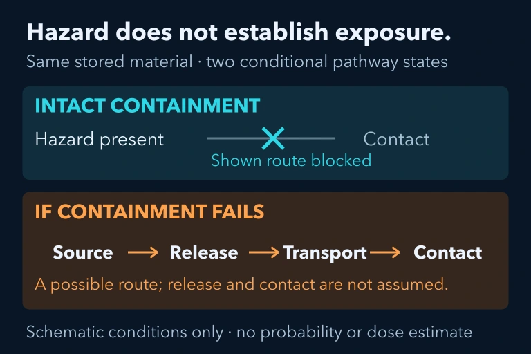Two pathways contrast blocked contact under intact containment with a conditional release–transport–contact sequence after failure. Intact containment can block exposure; failure permits release, transport and contact only if each pathway stage occurs.

SECTION 9

Practice Problems

Question 1: CONCEPTUAL

Substance X has an LD₅₀ of 25 mg/kg and Substance Y has an LD₅₀ of 400 mg/kg. Which of the following statements is correct?

A. Substance Y is more toxic because it has a larger LD₅₀ value.
B. Substance X is more toxic because a smaller dose kills 50% of the test population.
C. Substance X and Y are equally toxic because LD₅₀ only measures acute exposure.
D. Substance Y is more potent because more of it is required to cause a response.

Show answer (B)

B is correct. A lower LD₅₀ means less substance is needed to kill 50% of the test population, indicating greater acute toxicity. A is wrong because a larger LD₅₀ indicates lower toxicity, not higher. C is wrong because the two LD₅₀ values are clearly different, so the substances are not equally toxic; while LD₅₀ does measure acute exposure, that does not make them equal. D is wrong because requiring more substance to cause an effect means less potent, not more potent.

Question 2: BASIC CALCULATION

A pesticide has a NOAEL of 5 mg/kg/day from a chronic rat study. Using uncertainty factors of 10 for interspecies extrapolation and 10 for intraspecies variability, what is the reference dose (RfD)?

A. 0.5 mg/kg/day
B. 0.05 mg/kg/day
C. 50 mg/kg/day
D. 500 mg/kg/day

Show answer (B)

B is correct. RfD = NOAEL / (UF₁ × UF₂) = 5 / (10 × 10) = 5 / 100 = 0.05 mg/kg/day. A is wrong because it divides by only one uncertainty factor of 10 (5/10 = 0.5). C is wrong because it multiplies the NOAEL by 10 instead of dividing. D is wrong because it multiplies the NOAEL by 100 instead of dividing, reversing the formula entirely.

Question 3: INTERMEDIATE

A researcher plots dose-response curves for two chemicals, A and B, on the same graph. Chemical A has a steeper slope but a higher LD₅₀ than Chemical B. Which of the following is the best interpretation?

A. Chemical A is more toxic and affects all individuals at nearly the same dose.
B. Chemical B is more toxic, and Chemical A affects organisms over a narrower range of doses.
C. Chemical A has a lower threshold dose than Chemical B.
D. Both chemicals have equal potency because the curves appear on the same graph.

Show answer (B)

B is correct. Chemical B has the lower LD₅₀, making it more acutely toxic (its curve is shifted left). Chemical A's steeper slope means the population transitions from no response to full response over a narrow dose range, indicating uniform sensitivity — but slope and position on the x-axis measure different things. A is wrong because Chemical A has the higher LD₅₀ (less toxic, not more). C is wrong because a higher LD₅₀ does not imply a lower threshold. D is wrong because being on the same graph does not indicate equal potency; the x-axis positions differ.

Question 4: APPLIED

A scientist is studying the effects of mercury contamination on a fish population in a river downstream from a coal-burning power plant. Describe an investigation the scientist could design to determine the LC₅₀ of methylmercury for the fish species. Include the hypothesis, independent and dependent variables, a control, and how the results would be used to recommend a water quality standard.

Show answer

Point 1: A valid hypothesis states: "If the concentration of methylmercury in the water increases, then the percentage of fish that die within the 96-hour exposure period will increase." Point 2: The independent variable is the concentration of methylmercury in the water, tested at a minimum of five levels (e.g., 0.01, 0.05, 0.1, 0.5, 1.0 mg/L). The dependent variable is the percentage of fish that die after a standard 96-hour exposure. Each treatment should have multiple replicates with equal numbers of fish (e.g., 10 fish per tank, 3 replicates per concentration). Point 3: A control group consists of fish held in water with zero methylmercury under identical conditions — same temperature, dissolved oxygen, pH, tank dimensions, feeding regime, and fish of the same species, size, and age. Point 4: After plotting percentage mortality (y-axis) against methylmercury concentration (x-axis), the LC₅₀ is the concentration corresponding to 50% mortality on the resulting dose-response curve. This value would be divided by uncertainty factors (e.g., 10× for interspecies variation, 10× for sensitive subpopulations) to derive a recommended maximum contaminant level for methylmercury in the river.

Question 5: CRITICAL THINKING

The table below shows the results of a 96-hour LC₅₀ test for a new herbicide on Daphnia magna (water flea). Concentration (mg/L): 0 | 2 | 5 | 10 | 20 | 50 % Mortality: 0 | 5 | 20 | 55 | 85 | 100 (a) Estimate the LC₅₀ from the data. (b) The EPA wants to set a maximum contaminant level (MCL) for this herbicide in freshwater. Using the estimated LC₅₀ and a total safety factor of 1,000, calculate the MCL. (c) A farmer applies this herbicide near a stream, and subsequent water testing shows a concentration of 0.015 mg/L. Evaluate whether this concentration exceeds the MCL you calculated and discuss one potential ecological consequence if it does.

Show answer

(a) At 5 mg/L, mortality is 20%; at 10 mg/L, mortality is 55%. Since 50% falls between these two points, linear interpolation gives: LC₅₀ ≈ 5 + [(50 − 20) / (55 − 20)] × (10 − 5) = 5 + (30/35) × 5 ≈ 5 + 4.3 ≈ 9.3 mg/L. An estimate of approximately 8–9 mg/L is also acceptable depending on interpolation method. (b) MCL = LC₅₀ / safety factor = 9.3 / 1,000 = 0.0093 mg/L. Using LC₅₀ ≈ 8.5 mg/L would yield MCL = 0.0085 mg/L. (c) The measured concentration of 0.015 mg/L exceeds the calculated MCL of ~0.009 mg/L by roughly 1.5–1.8 times. This exceedance poses ecological risk: Daphnia are keystone grazers in freshwater ecosystems, and their decline would reduce grazing pressure on algae, potentially triggering algal blooms. Algal blooms can deplete dissolved oxygen (leading to hypoxia), harming fish and other aquatic organisms — a cascading trophic disruption.