Bioaccumulation and Biomagnification - AP Environmental Science

SECTION 1

Historical Context & Motivation

The realization that synthetic chemicals could travel through entire food webs—concentrating to dangerous levels in top predators—was one of the most consequential insights in twentieth-century environmental science. Before the 1950s, regulators assumed that diluting a contaminant in a large body of water rendered it harmless, because ambient concentrations were orders of magnitude below acute toxicity thresholds. That assumption proved catastrophically wrong when scientists discovered that organisms at the top of aquatic and terrestrial food chains were accumulating certain persistent organic pollutants (POPs) at concentrations millions of times higher than those found in surrounding water or soil. The ecological and human health consequences of this phenomenon reshaped pesticide regulation, catalyzed the modern environmental movement, and remain a central topic on the AP Environmental Science exam.

1939 • DDT Synthesized for Insect Control

Paul Hermann Müller demonstrated that DDT was a potent insecticide; its widespread agricultural and military use began shortly afterward, eventually earning Müller the Nobel Prize in 1948.

1962 • Silent Spring Published

Rachel Carson's landmark book documented how DDT biomagnified through food chains, causing reproductive failure in birds of prey such as bald eagles and peregrine falcons via eggshell thinning.

1972 • U.S. DDT Ban

The newly formed EPA banned most uses of DDT in the United States, citing unacceptable ecological risks, particularly to nontarget species at higher trophic levels.

2001 • Stockholm Convention on POPs

An international treaty targeted twelve initial POPs (the 'dirty dozen') for elimination or restriction, formally recognizing that bioaccumulation and biomagnification pose global threats to ecosystem and human health.

2017 • Minamata Convention Enters Force

The global treaty to reduce mercury emissions entered into force, directly addressing the bioaccumulation of methylmercury in aquatic food webs and the resulting human health crises.

This historical trajectory raises the central question that this lesson addresses: why do certain contaminants become more concentrated as they move from the environment into organisms, and then from lower trophic levels to higher ones? Understanding the mechanisms behind bioaccumulation and biomagnification is essential for predicting which pollutants pose the greatest ecological risk and for designing effective regulatory strategies.

SECTION 2

Core Principles & Definitions

Two closely related but distinct processes govern how pollutants concentrate in living systems. Although often confused on exams, each operates at a different scale and through a different mechanism; precise definitions are critical for earning full credit on both the multiple-choice and free-response sections of the AP Environmental Science exam.

Bioaccumulation

The net increase in concentration of a substance in an individual organism over time. It occurs because the rate of uptake (via respiration, ingestion, or dermal absorption) exceeds the rate of metabolic breakdown plus excretion.

Biomagnification

The progressive increase in the concentration of a substance across successive trophic levels in a food chain. Each consumer ingests many prey items, each already carrying a bioaccumulated load, so the predator's tissue concentration can be orders of magnitude higher.

Bioconcentration

A subset of bioaccumulation that refers specifically to the uptake of a chemical directly from the abiotic environment (usually water) through respiratory or dermal surfaces, without dietary intake. This is often measured in controlled lab settings.

Persistence & Lipophilicity

Chemicals most prone to bioaccumulation are persistent (resistant to chemical, biological, and photolytic degradation) and lipophilic (fat-soluble), meaning they partition into fatty tissues rather than being dissolved in water and excreted.

Trophic Transfer Efficiency

Only about 10% of energy transfers between trophic levels (the ten percent rule), but a far larger fraction of a lipophilic pollutant transfers, because the contaminant is stored in fat rather than being metabolized for energy.

✦

KEY TAKEAWAY

Think of bioaccumulation like a bathtub with the drain partially blocked: water flows in faster than it drains out, so the level rises steadily over time. Biomagnification is what happens when a series of progressively larger bathtubs are connected—each downstream tub receives the overflow from many smaller ones, so the water level in each successive tub is dramatically higher. In biological terms, each predator is a larger 'tub' fed by many contaminated prey items, and the contaminant 'water level' in its tissues keeps climbing with each trophic step.

SECTION 3

Visual Explanation — The Food-Chain Amplification Model

The diagram above illustrates biomagnification of DDT through an aquatic food chain. Notice how the DDT tissue concentration increases by roughly one order of magnitude at each trophic level: from 0.000003 ppm in water to 25 ppm in the top predator—a magnification factor of approximately 8.3 million relative to the ambient water concentration.

Several features of this diagram deserve close attention. First, the water concentration of DDT is extraordinarily low—parts per trillion—yet the top predator carries concentrations in the parts-per-million range. This occurs because each organism ingests many contaminated prey items over its lifetime, and DDT's high lipophilicity means it is sequestered in adipose tissue rather than being metabolized or excreted efficiently. Second, the arrows point upward through the food chain, reinforcing that biomagnification is a trophic-level phenomenon: the contaminant increases in concentration at each step not because the predator is exposed to more contaminated water, but because it consumes many organisms that have themselves already bioaccumulated the pollutant.

SECTION 4

Mathematical Framework

While the AP Environmental Science exam rarely asks students to perform complex calculations involving bioaccumulation kinetics, a quantitative understanding of the key indices strengthens conceptual reasoning and is essential for free-response questions that involve data analysis. Two metrics are central: the bioconcentration factor (BCF) and the biomagnification factor (BMF).

BIOCONCENTRATION FACTOR

BCF = C_organism / C_water

Where C_organism is the concentration of the contaminant in the organism's tissue (mg/kg) and C_water is the concentration in the surrounding water (mg/L). A BCF > 1 indicates the organism concentrates the chemical above ambient levels; BCF > 5,000 is classified as highly bioaccumulative under EPA criteria.

BIOMAGNIFICATION FACTOR

BMF = C_predator / C_prey

Where C_predator is the tissue concentration in the consumer and C_prey is the tissue concentration in its prey. A BMF > 1 confirms that the substance biomagnifies (i.e., its concentration increases from one trophic level to the next).

OVERALL MAGNIFICATION ACROSS n TROPHIC LEVELS

C_n = C_water × BCF × BMF^(n−1)

This simplified model assumes a constant BMF at each trophic step. C_n is the concentration at trophic level n, BCF accounts for the initial uptake by the producer from water, and BMF⁽ⁿ⁻¹⁾ accounts for successive trophic transfers. In reality, BMF varies between trophic steps.

The octanol-water partition coefficient (K_ow) is a laboratory measurement that predicts a chemical's tendency to bioaccumulate. K_ow quantifies how a chemical partitions between a lipophilic phase (octanol) and water; substances with log K_ow > 5 are strongly lipophilic and highly likely to bioaccumulate. DDT, for instance, has a log K_ow of approximately 6.9, explaining its extreme bioaccumulative potential.

SECTION 5

Key Pollutants That Bioaccumulate and Biomagnify

Not all pollutants bioaccumulate or biomagnify. The chemicals that pose the greatest risk share two properties: they are persistent (they resist degradation and remain in the environment for years to decades) and lipophilic (they dissolve readily in fats and oils, allowing them to be stored in adipose tissue rather than excreted in urine). The table below summarizes the most commonly tested pollutants on the APES exam and their ecological consequences.

Pollutant	Class	Primary Source	Ecological Effect of Biomagnification
DDT / DDE	Organochlorine pesticide	Agricultural spraying; still used in some regions for malaria control	Eggshell thinning in raptors via disruption of calcium metabolism; population crashes in bald eagles, peregrine falcons, and brown pelicans
Mercury (as methylmercury)	Heavy metal	Coal combustion; artisanal gold mining; volcanic emissions	Neurotoxicity in fish-eating mammals and birds; developmental impairment in human fetuses (Minamata disease)
PCBs	Synthetic industrial chemical	Electrical transformers, coolants; legacy contamination in river sediments	Immune suppression, reproductive failure, and endocrine disruption in marine mammals such as orcas and beluga whales
PFAS	Per- and polyfluoroalkyl substances	Firefighting foam (AFFF), nonstick coatings, food packaging	Liver damage, immune suppression; sometimes called 'forever chemicals' because they resist virtually all forms of degradation
Lead	Heavy metal	Lead ammunition in hunting, legacy lead paint and gasoline, mining waste	Lead poisoning in scavengers such as California condors that consume carcasses with embedded lead shot fragments

Major bioaccumulative pollutants tested on the APES exam

This scatterplot positions common environmental contaminants by their lipophilicity (log K_ow) on the x-axis and environmental persistence on the y-axis. The red dashed box highlights the 'high risk zone' where substances such as DDT, PCBs, and PFAS combine high lipophilicity with extreme persistence—the two properties most predictive of biomagnification.

SECTION 6

Worked Example — Calculating Biomagnification

A lake ecosystem is contaminated with mercury. Scientists measure the following methylmercury concentrations: water = 0.001 ppm; phytoplankton = 0.5 ppm; zooplankton = 2.0 ppm; small fish = 8.0 ppm; large fish = 40.0 ppm; osprey = 200.0 ppm. Let us calculate several indices of bioaccumulation and biomagnification.

Mercury Biomagnification in a Lake Food Chain

1
Step 1 — Calculate the BCF for phytoplankton

BCF = C_organism / C_water = 0.5 ppm / 0.001 ppm

BCF = 500 — phytoplankton concentrate mercury 500× above ambient water levels.
2
Step 2 — Calculate the BMF from zooplankton to small fish

BMF = C_predator / C_prey = 8.0 ppm / 2.0 ppm

BMF = 4 — small fish carry 4× the mercury concentration of zooplankton.
3
Step 3 — Calculate the overall magnification factor from water to osprey

Overall magnification = C_osprey / C_water = 200.0 ppm / 0.001 ppm

Overall magnification = 200,000× — the osprey has mercury concentrations 200,000 times greater than the ambient water.
4
Step 4 — Interpret ecological significance

Mercury concentrations above approximately 0.5 ppm in fish tissue trigger human health advisories, and concentrations above 20 ppm in bird tissue are associated with reproductive impairment. At 200 ppm, the osprey is well above the threshold for severe neurological and reproductive effects. This illustrates why even trace-level mercury contamination in water bodies can produce lethal concentrations in top predators through biomagnification.

SECTION 7

Factors Influencing Bioaccumulation — and Model Limitations

The simplified equations presented in Section 4 assume uniform BMF values across trophic levels and stable environmental conditions, but real ecosystems introduce substantial complexity. Several biological, chemical, and ecological factors influence the degree to which a contaminant accumulates and magnifies. Understanding these factors helps explain why bioaccumulation is not a fixed property of a chemical but rather an emergent outcome of organism–environment interactions.

Factor	Effect on Bioaccumulation	Limitation of Simple Models
Metabolic rate	Organisms with higher metabolic rates may excrete contaminants faster, reducing bioaccumulation. Warm-blooded species often have lower BCFs for some compounds than cold-blooded ones.	Constant-BMF models ignore species-specific metabolism
Organism age & body size	Older and larger organisms have longer exposure histories, so they tend to carry higher body burdens of persistent pollutants.	Models assume steady-state rather than time-dependent accumulation
Lipid content	Species with higher body-fat percentages store more lipophilic pollutants. Marine mammals such as orcas and polar bears carry extremely high pollutant loads due to thick blubber layers.	Simple models do not normalize concentrations to lipid weight
Food-web complexity	Organisms that feed at multiple trophic levels (omnivores) or that shift diet seasonally complicate the linear-chain model of biomagnification.	Linear food-chain models oversimplify real food webs
Chemical speciation	The chemical form matters: inorganic mercury is relatively poorly absorbed, while methylmercury (produced by anaerobic bacteria) is efficiently absorbed and highly biomagnified.	Models that treat all forms of a metal as equivalent miss critical differences in bioavailability

Factors influencing bioaccumulation and limitations of simplified models

✦

KEY TAKEAWAY

Bioaccumulation and biomagnification are not mechanical certainties—they are probabilistic outcomes shaped by the interplay of a chemical's physical properties and the biological characteristics of each species in the food web. The simple BMF model is useful for estimation and exam calculations, but real-world risk assessment requires species-specific data, food-web topology, and consideration of chemical speciation. Think of the model as a first-order approximation analogous to the ideal gas law in chemistry: useful and often directionally correct, but incomplete in complex systems.

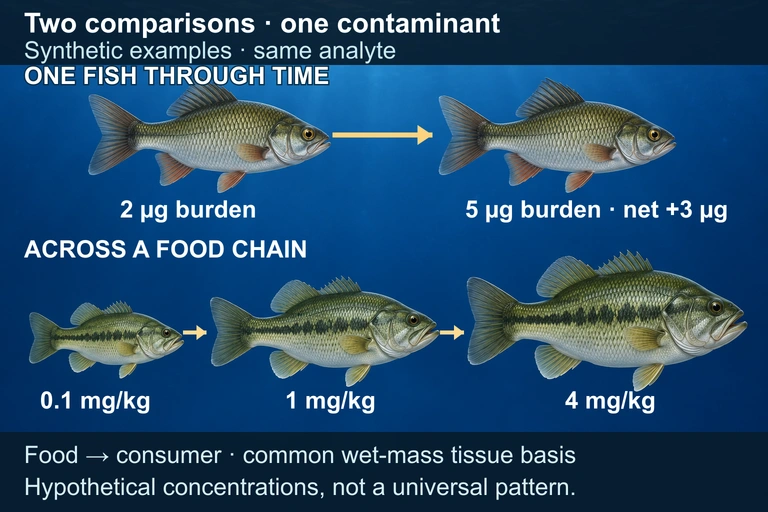Two equal-size fish symbols compare one fish at two times,with tissue burden rising from2 to5 micrograms. A separate row shows three feeding-level fish symbols with synthetic tissue concentrations0.1,1 and4mg/kg on the same measurement basis. Bioaccumulation tracks uptake and loss within an organism over time. Biomagnification compares tissue concentrations across feeding relationships on a common measurement basis.

SECTION 8

Policy Responses & Advanced Connections

Understanding bioaccumulation and biomagnification has driven some of the most significant environmental policies of the past half-century. Because the consequences of these processes are often separated in time and space from the point of contamination, regulatory frameworks must be proactive rather than reactive. This section connects the scientific concepts to the policy tools most commonly addressed on the APES exam and in college-level environmental science courses.

Policy / Regulation	Mechanism	Connection to Bioaccumulation / Biomagnification
Stockholm Convention (2001)	International treaty banning or restricting POPs	Targets chemicals specifically because they are persistent, bioaccumulative, toxic, and capable of long-range transport
Clean Water Act (1972)	Sets effluent limits and water quality criteria for toxic pollutants	Water quality criteria for bioaccumulative pollutants (e.g., mercury) are set far lower than acute toxicity thresholds to account for food-chain amplification
EPA Fish Consumption Advisories	Informs public about mercury and PCB levels in locally caught fish	Advisories directly address human exposure to biomagnified contaminants via dietary intake of top-predator fish (tuna, swordfish, bass)
Minamata Convention (2013/2017)	International treaty phasing down mercury use and emissions	Named after Minamata Bay disaster where methylmercury biomagnification caused mass neurological poisoning; directly motivated by food-chain concentration
Bioremediation & Phytoremediation	Uses organisms (bacteria, plants) to extract or degrade contaminants	Plants that hyperaccumulate heavy metals can be used to remove contaminants from soil, exploiting bioaccumulation as a remediation tool rather than a hazard

Key policies addressing bioaccumulation and biomagnification

Looking forward, the emergence of PFAS contamination represents a new frontier in bioaccumulation science. Unlike the classic lipophilic POPs, some PFAS compounds are both hydrophobic and oleophobic, binding to proteins rather than lipids, which challenges traditional BCF models calibrated to lipid partitioning. Additionally, microplastics are increasingly recognized as vectors for bioaccumulative contaminants: persistent organic pollutants adsorb onto microplastic surfaces and may be released during digestion, potentially increasing the bioavailability of toxicants to marine organisms. These evolving challenges ensure that bioaccumulation and biomagnification will remain at the forefront of environmental science for decades to come.

SECTION 9

Practice Problems

Question 1: CONCEPTUAL

A scientist measures the concentration of a pesticide in the tissues of organisms at four trophic levels of an aquatic food chain. The pesticide concentration is highest in tertiary consumers and lowest in producers. Which of the following best explains this pattern?

A. Tertiary consumers have the fastest metabolic rates, so they absorb more of the pesticide from water.
B. The pesticide is water-soluble and is concentrated by the kidneys of higher-level consumers.
C. Each consumer ingests many prey organisms that have already bioaccumulated the persistent, lipophilic pesticide, so the concentration increases at each trophic level.
D. Producers actively pump the pesticide out of their cells, making them appear to have lower concentrations.

Show answer (C)

C is correct. Biomagnification occurs because each consumer eats many prey items, each carrying a bioaccumulated load of a persistent, fat-soluble pollutant. The contaminant is stored in adipose tissue rather than being metabolized or excreted, so tissue concentrations increase at each successive trophic level. A is incorrect because metabolic rate alone does not explain trophic-level increases; in fact, higher metabolic rates can increase excretion. B is incorrect because water-soluble chemicals are readily excreted and typically do NOT biomagnify. D is incorrect because producers do not actively pump out pesticides; the pattern is due to trophic accumulation, not producer exclusion.

Question 2: BASIC CALCULATION

The methylmercury concentration in a lake is 0.002 ppm. Algae in the lake contain methylmercury at 1.0 ppm. Small fish that eat the algae have a methylmercury concentration of 5.0 ppm. What is the biomagnification factor (BMF) from algae to small fish?

A. 500
B. 2,500
C. 5
D. 0.2

Show answer (C)

C is correct. BMF = C_predator / C_prey = 5.0 ppm / 1.0 ppm = 5. The BMF compares concentrations between adjacent trophic levels (predator vs. prey), NOT between the organism and the water. A (500) is the BCF for algae relative to water (1.0/0.002), conflating bioconcentration with biomagnification. B (2,500) divides the small fish concentration by the water concentration, which gives the overall bioconcentration factor, not the BMF. D (0.2) inverts the ratio (prey/predator), which would incorrectly suggest biodilution.

Question 3: INTERMEDIATE

Two lakes have identical dissolved mercury concentrations. Lake A has a simple food chain with three trophic levels (phytoplankton → zooplankton → bass). Lake B has five trophic levels (phytoplankton → zooplankton → minnows → bass → osprey). Assuming equal BMFs at each trophic step, which lake would be expected to have higher mercury concentrations in its top predator, and why?

A. Lake A, because shorter food chains concentrate pollutants more efficiently
B. Lake B, because more trophic levels provide more opportunities for biomagnification
C. Both lakes would have equal mercury in top predators because the dissolved mercury concentration is the same
D. Lake A, because bass in a shorter food chain eat more total prey over their lifetime

Show answer (B)

B is correct. Biomagnification is a multiplicative process: at each trophic step, the concentration increases by the BMF. Using the formula C_n = C_water × BCF × BMF⁽ⁿ⁻¹⁾, a five-level chain yields BMF⁴ while a three-level chain yields BMF². With more trophic steps, the top predator in Lake B has a substantially higher body burden. A and D are incorrect because shorter food chains produce less biomagnification, not more. C is incorrect because equal water concentrations do not produce equal top-predator concentrations when food-chain length differs.

Question 4: APPLIED

4 pts

A team of researchers suspects that mercury is biomagnifying in a freshwater lake ecosystem. Design an investigation to test the hypothesis that methylmercury concentrations increase with trophic level. (a) State a testable hypothesis. (1 point) (b) Describe the data collection procedure, including what organisms would be sampled and what measurements would be taken. (1 point) (c) Identify one variable that must be controlled and explain why. (1 point) (d) Describe how the data would be analyzed to determine whether biomagnification is occurring. (1 point)

Show answer

Rubric — 4 points total: (a) Hypothesis (1 point): The student earns 1 point for a testable hypothesis that relates methylmercury tissue concentration to trophic level. Example: 'If methylmercury biomagnifies in this freshwater lake ecosystem, then organisms at higher trophic levels will have significantly higher tissue concentrations of methylmercury than organisms at lower trophic levels.' (b) Data collection (1 point): The student earns 1 point for describing a procedure that includes: collecting tissue samples from organisms at a minimum of three different trophic levels (e.g., phytoplankton, zooplankton, small planktivorous fish, large piscivorous fish); using multiple individuals per species for replication; and measuring methylmercury concentration (e.g., in mg/kg or ppm) in tissue using chemical analysis such as atomic absorption spectroscopy. Water samples should also be collected to establish a baseline ambient mercury concentration. (c) Controlled variable (1 point): The student earns 1 point for identifying a relevant controlled variable and explaining its importance. Examples include: tissue type analyzed (e.g., muscle vs. liver, since different organs accumulate mercury at different rates); organism age or size class within a species (older or larger individuals have had longer exposure time and thus greater bioaccumulation); or time of year of sampling (seasonal variation in lipid content and feeding behavior can affect mercury concentrations). The student must explain why controlling this variable is necessary to ensure valid comparisons across trophic levels. (d) Data analysis (1 point): The student earns 1 point for describing an appropriate analytical approach. Example: Calculate the mean methylmercury concentration for each trophic level and create a bar graph or scatterplot of concentration versus trophic level. Calculate the biomagnification factor (BMF) between adjacent trophic levels by dividing the mean concentration at the higher trophic level by the mean concentration at the lower trophic level. If the BMF is greater than 1 at each successive trophic level and concentrations show a statistically significant increasing trend across trophic levels, the hypothesis that biomagnification is occurring is supported.

Question 5: CRITICAL THINKING

4 pts

The following data were collected from an estuary contaminated with PCBs: Water: 0.00005 ppm Phytoplankton: 0.05 ppm Mussels (filter feeders): 1.0 ppm Small fish: 4.0 ppm Striped bass: 20.0 ppm Osprey: 80.0 ppm (a) Calculate the bioconcentration factor (BCF) for phytoplankton relative to water. (1 point) (b) Calculate the biomagnification factor (BMF) from striped bass to osprey. (1 point) (c) Explain why filter-feeding mussels might have a higher tissue concentration than expected based solely on their trophic position as primary consumers. (1 point) (d) A nearby factory has reduced its PCB discharge by 95%. Predict and justify whether PCB concentrations in osprey tissue would decline immediately, and explain one factor that could delay recovery. (1 point)

Show answer

Rubric — 4 points total: (a) BCF calculation (1 point): BCF = C_{phytoplankton} / C_water = 0.05 / 0.00005 = 1,000. The student earns 1 point for the correct setup and answer. (b) BMF calculation (1 point): BMF = C_osprey / C_bass = 80.0 / 20.0 = 4. The student earns 1 point for the correct setup and answer. (c) Filter feeder explanation (1 point): Mussels are filter feeders that process enormous volumes of water daily, extracting suspended particles (including phytoplankton and organic matter to which PCBs adsorb). This high filtration rate exposes them to a disproportionately large mass of contaminant relative to their body size, resulting in higher bioaccumulation than would be predicted by trophic position alone. Additionally, PCBs adsorbed to sediment particles are filtered and ingested, adding another exposure pathway beyond diet. (d) Prediction and justification (1 point): Osprey tissue PCB concentrations would NOT decline immediately. PCBs are highly persistent and lipophilic (they are stored in fat and have biological half-lives of years to decades). Even after discharge is reduced, legacy PCBs remain stored in sediments and in the tissues of organisms throughout the food web. One key factor delaying recovery is the release of PCBs from contaminated sediments during storm events or bioturbation, which re-introduces the pollutant into the water column and food web long after the source discharge has ceased. The long lifespan of top predators like osprey also means that individuals accumulated PCBs over many years and will continue to carry those body burdens.

SUMMARY

Summary

Bioaccumulation is the process by which an individual organism accumulates a contaminant in its tissues over time because uptake exceeds excretion and metabolic breakdown. Biomagnification extends this phenomenon across trophic levels: because each predator consumes many contaminated prey items, tissue concentrations increase progressively up the food chain. The chemicals most susceptible to these processes are persistent (resistant to degradation) and lipophilic (fat-soluble), such as DDT, PCBs, methylmercury, and PFAS.

Quantitatively, the bioconcentration factor (BCF) measures the ratio of tissue concentration to water concentration, while the biomagnification factor (BMF) measures the increase from prey to predator. Key factors that influence these processes include organism metabolic rate, body lipid content, food-chain length, and the chemical speciation of the contaminant. Policy responses—from Rachel Carson's Silent Spring to the Stockholm Convention and Minamata Convention—have directly targeted bioaccumulative pollutants, and understanding these mechanisms is essential for evaluating both the ecological impacts of contamination and the design of effective remediation strategies.