Aquatic Biomes - AP Environmental Science

SECTION 1

Historical Context & Motivation

Long before scientists formalized the concept of a biome, coastal and riverine communities understood that water bodies differ dramatically in the life they support. Greek natural philosophers such as Aristotle cataloged marine organisms by habitat zone, while Polynesian navigators recognized distinct pelagic provinces based on current patterns and species assemblages. The modern study of aquatic biomes emerged as limnology and oceanography matured into rigorous disciplines during the nineteenth and twentieth centuries, driven by the need to understand fisheries, water quality, and global biogeochemical cycling.

1872 • HMS Challenger Expedition

The first global oceanographic survey mapped seafloor topography, measured water chemistry, and cataloged thousands of marine species, establishing the physical framework for ocean biome classification.

1935 • Tansley Coins 'Ecosystem'

Arthur Tansley introduced the ecosystem concept, providing the theoretical basis for treating aquatic habitats as integrated units of biotic communities and abiotic factors.

1953 • Odum's Energy-Flow Studies

Eugene Odum and Howard T. Odum quantified energy flow in Silver Springs, Florida, pioneering systems ecology and demonstrating how productivity varies across freshwater and marine systems.

1975 • Whittaker's Biome Classification

Robert Whittaker's climatic biome scheme, originally terrestrial, was extended by limnologists and marine ecologists to classify aquatic biomes by salinity, depth, light penetration, and flow.

2005 • Millennium Ecosystem Assessment

A landmark UN report documented that aquatic ecosystems provide ecosystem services worth trillions of dollars annually and face accelerating degradation from pollution, overfishing, and climate change.

These milestones reveal a persistent question that still guides AP Environmental Science: what abiotic factors determine which organisms thrive in a given body of water, and how do human activities alter those factors? Answering that question requires a systematic classification of Earth's aquatic environments—freshwater, marine, and the transitional zones that bridge them.

SECTION 2

Core Principles & Definitions

Aquatic biomes are classified primarily by salinity (freshwater < 0.5 ppt; marine ~35 ppt; brackish in between) and secondarily by physical characteristics such as depth, light availability, flow rate, and temperature. Unlike terrestrial biomes, which are defined largely by temperature and precipitation, aquatic biomes depend on the chemical and physical properties of water itself—its high specific heat, density behavior, and capacity to dissolve gases and nutrients.

Salinity Gradient

The dissolved salt concentration separates freshwater systems (lakes, rivers, wetlands) from marine systems (oceans, coral reefs). Estuaries occupy the transition zone where salinity fluctuates with tides.

Photic vs. Aphotic Zones

Sunlight penetrates only the upper ~200 m of open water (the photic zone). Below this, the aphotic zone relies on chemosynthesis or a rain of organic detritus for energy inputs.

Lentic vs. Lotic

Standing (lentic) waters like lakes and ponds develop thermal stratification. Flowing (lotic) waters like rivers and streams are shaped by current velocity, gradient, and substrate type.

Dissolved Oxygen & Nutrients

Oxygen solubility decreases with rising temperature and salinity. Nutrient availability (N, P) drives productivity and can cause eutrophication when anthropogenically enriched.

Benthic vs. Pelagic

The benthic zone encompasses the bottom substrate and its attached communities. The pelagic zone is the open water column, subdivided by depth into neritic (nearshore) and oceanic provinces.

SECTION 3

Visual Explanation — Aquatic Biome Zonation

Ocean zones are defined by depth and light availability. The epipelagic (photic) zone supports photosynthesis and contains the bulk of marine biodiversity. The neritic province over the continental shelf is distinct from the open oceanic province beyond it.

The diagram illustrates the vertical structure of the open ocean, the single largest biome on Earth by area. Notice that light penetration controls the fundamental division: only the upper photic zone receives enough photosynthetically active radiation (PAR) to support primary producers like phytoplankton and macroalgae. Below the aphotic zone threshold (~200 m), organisms depend on sinking organic matter—sometimes called marine snow—or on chemosynthetic bacteria near hydrothermal vents. Horizontally, the neritic zone overlying the continental shelf supports higher productivity due to nutrient runoff and upwelling, while the oceanic zone is nutrient-poor but vast.

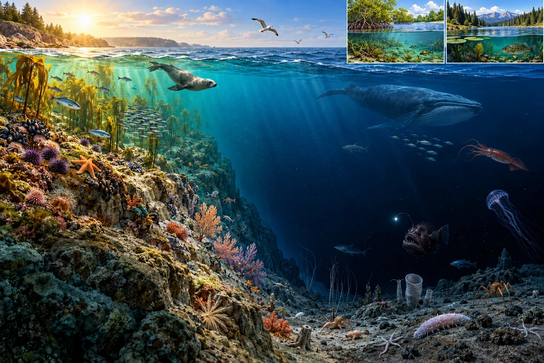A coastal-to-deep ocean cutaway with kelp, fish and marine mammals, continuous seafloor, and separate mangrove and lake insets. Nearshore and offshore describe horizontal position; photic and aphotic describe light conditions. Benthic habitat is the seafloor at any depth.

Aquatic zones use different spatial dimensions. Nearshore and offshore describe horizontal position; photic and aphotic describe light conditions. Benthic habitat is the seafloor at any depth. 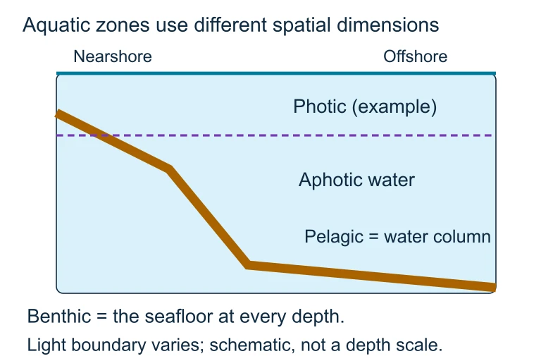Nearshore and offshore describe horizontal position; photic and aphotic describe light conditions. Benthic habitat is the seafloor at any depth.

SECTION 4

How Abiotic Factors Shape Aquatic Biomes

Thermal Stratification in Lakes

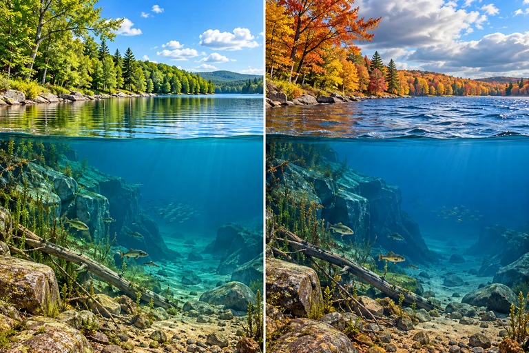
Temperature exerts profound control over aquatic ecosystems. In temperate lakes, solar heating warms the surface layer (epilimnion) while deeper water (hypolimnion) remains cold and dense. Separating them is the thermocline (or metalimnion), a narrow zone of rapid temperature change. This thermal stratification restricts vertical mixing and traps nutrients in the hypolimnion during summer. Twice a year—in spring and autumn—surface temperatures converge with bottom temperatures, erasing the density gradient and allowing full-lake turnover that redistributes dissolved oxygen and nutrients. This mixing pulse drives seasonal algal blooms and is a defining feature of dimictic lakes.

Net Primary Productivity in Aquatic Systems

NET PRIMARY PRODUCTIVITY

NPP = GPP − R

NPP = net primary productivity (g C m⁻² yr⁻¹); GPP = gross primary productivity; R = autotroph respiration. In aquatic biomes, NPP is strongly limited by light and nutrient availability.

LIGHT ATTENUATION (BEER–LAMBERT LAW)

I(z) = I₀ × e^(−k × z)

I(z) = light intensity at depth z; I₀ = surface irradiance; k = attenuation coefficient (m⁻¹), which increases with turbidity and dissolved organic matter; z = depth (m). The photic zone ends where I(z) ≈ 1% of I₀.

The Beer–Lambert relationship explains why turbid estuaries have shallow photic zones while clear oligotrophic lakes allow light to penetrate much deeper. A high k value—caused by suspended sediment, algal cells, or dissolved organics—collapses the photic zone and limits where photosynthesis can occur. This directly links water clarity to ecosystem productivity and biome classification.

Salinity & Osmotic Stress

Salinity determines organism distribution more than almost any other single factor. Freshwater organisms maintain internal ion concentrations higher than their surroundings and must actively excrete excess water, while marine species face the opposite osmotic challenge. Species adapted to estuarine conditions (euryhaline species) possess specialized ion-transport mechanisms, but most aquatic organisms are stenohaline—tolerant of only a narrow salinity range. This physiological constraint is why the freshwater–marine boundary constitutes a major biogeographic barrier.

Matched summer and autumn lake cutaways accompany temperature-versus-depth profiles on the same axes. The summer profile has warm surface water above colder deep water. In autumn, a weaker density difference allows mixing when sufficient wind energy is available.

A thermal gradient can resist mixing. The summer profile has warm surface water above colder deep water. In autumn, a weaker density difference allows mixing when sufficient wind energy is available. 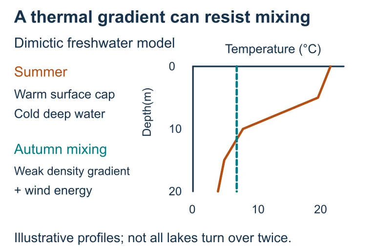The summer profile has warm surface water above colder deep water. In autumn, a weaker density difference allows mixing when sufficient wind energy is available.

SECTION 5

Freshwater, Marine & Transitional Biomes

The three major categories of aquatic biomes—freshwater, transitional, and marine—each contain distinct habitat types defined by physical structure, flow, and salinity.

Biome Type	Key Abiotic Factors	Dominant Producers	Relative NPP
Oligotrophic Lake	Low nutrients, clear water, deep photic zone	Sparse phytoplankton, littoral macrophytes	Low
Eutrophic Lake	High nutrients, turbid, shallow photic zone	Dense phytoplankton, cyanobacteria blooms	High
River / Stream	Flow velocity, dissolved O₂, substrate	Periphyton, riparian inputs (allochthonous)	Low–Moderate
Estuary	Fluctuating salinity, tidal mixing, sediment load	Salt-tolerant grasses, phytoplankton, algae	Very High
Coral Reef	Warm (23–29 °C), clear, shallow, high light	Zooxanthellae (symbiotic dinoflagellates)	Very High
Open Ocean	Nutrient-poor surface, vast area, deep	Phytoplankton (diatoms, coccolithophores)	Low per m², huge total

Comparison of major aquatic biome types by abiotic factors, producers, and productivity

SECTION 6

Worked Example — Photic Zone Depth & Eutrophication

A common AP Environmental Science task requires students to connect anthropogenic nutrient loading to changes in aquatic biome structure. The following worked example uses the Beer–Lambert light-attenuation model to show how eutrophication shrinks the photic zone.

Worked example

1
Step 1 — Identify Given Values

A clear oligotrophic lake has an attenuation coefficient k = 0.05 m⁻¹. After years of agricultural runoff, algal growth increases turbidity and k rises to 0.20 m⁻¹. Surface irradiance I₀ = 1 000 µmol photons m⁻² s⁻¹. The photic zone ends where I(z) = 1% of I₀ = 10 µmol photons m⁻² s⁻¹.
2
Step 2 — Apply Beer–Lambert Law (Before Runoff)

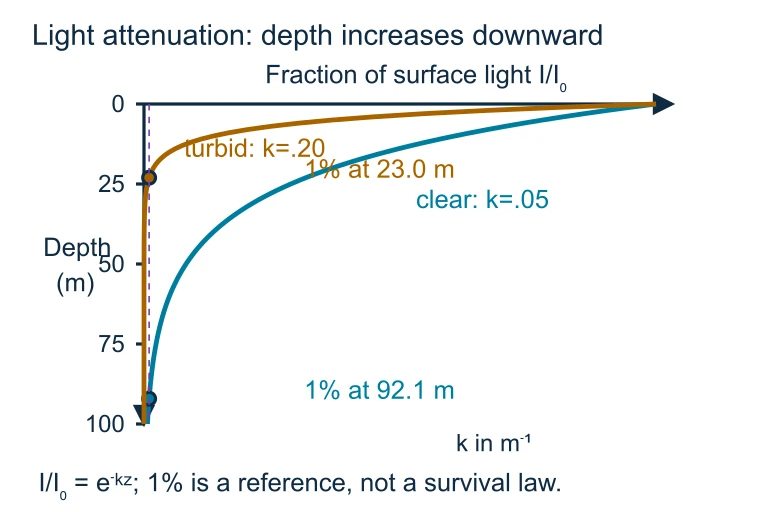
Set I(z) = 0.01 × I₀ and solve for z: 0.01 = $e^{−0.05 × z}$ . Taking the natural log: ln(0.01) = −0.05z → −4.605 = −0.05z → z = 92.1 m.

Photic zone (before) ≈ 92 m
3
Step 3 — Apply Beer–Lambert Law (After Runoff)

With k = 0.20 m⁻¹: ln(0.01) = −0.20z → −4.605 = −0.20z → z = 23.0 m.

Photic zone (after) ≈ 23 m
4
Step 4 — Interpret Ecological Impact

The photic zone shrank by about 75%—from 92 m to 23 m. This means photosynthesis is now confined to the upper quarter of the water column. Submerged aquatic vegetation (SAV) on the lake bottom below 23 m will die, benthic oxygen demand will increase as dead plant material decomposes, and the lake may shift from an oligotrophic to a eutrophic state with hypoxic bottom waters.

Eutrophication reduces photic zone depth → loss of SAV → potential hypoxia

Two complete underwater scenes with a diver, one clear blue and one turbid, with differing penetration of visible sunlight. Using the stated light-attenuation model, the 1% surface-light reference occurs at 92.1 m when k = 0.05 m⁻¹ and 23.0 m when k = 0.20 m⁻¹. Light requirements vary among organisms.

Light attenuation: depth increases downward. Using the stated light-attenuation model, the 1% surface-light reference occurs at 92.1 m when k = 0.05 m⁻¹ and 23.0 m when k = 0.20 m⁻¹. Light requirements vary among organisms. Using the stated light-attenuation model, the 1% surface-light reference occurs at 92.1 m when k = 0.05 m⁻¹ and 23.0 m when k = 0.20 m⁻¹. Light requirements vary among organisms.

SECTION 7

Ecosystem Services & Threats

Aquatic Biome	Key Ecosystem Services	Primary Threats
Freshwater Wetlands	Flood mitigation, water filtration, carbon storage, nursery habitat	Draining for agriculture, urban development, invasive species
Rivers & Streams	Drinking water, irrigation, sediment transport, recreation	Damming, channelization, pollution, water diversion
Estuaries	Fisheries nursery (>75% of commercial species), nutrient cycling	Nutrient loading, coastal development, hypoxic dead zones
Coral Reefs	Biodiversity hotspot, coastal protection, tourism, fisheries	Ocean warming (bleaching), acidification, sedimentation, overfishing
Open Ocean	O₂ production (~50% of global), CO₂ absorption, fisheries, climate regulation	Overfishing, plastic pollution, ocean acidification, deoxygenation

Ecosystem services and anthropogenic threats for major aquatic biomes

SECTION 8

Connections to Global Environmental Issues

Aquatic biomes do not exist in isolation; they are embedded within the larger Earth system and are affected by, and contribute to, global environmental challenges studied throughout the AP Environmental Science curriculum. Understanding these connections is essential for FRQ responses that require you to trace cause-and-effect chains across multiple units.

Concept in This Lesson	Connection to Broader APES Topic
Eutrophication & hypoxic zones	Unit 8: Nutrient pollution from agriculture; Gulf of Mexico dead zone; Clean Water Act
Coral bleaching	Unit 9: Climate change; ocean warming; CO₂ → carbonic acid → lower pH
Wetland loss	Unit 5: Land use change; loss of carbon sinks; flood risk increases
Thermohaline circulation	Unit 4: Global water cycle; heat transport; climate regulation
Invasive species in freshwater	Unit 2: Biodiversity; zebra mussels; trophic cascades

ℹ

EXAM TIP

SECTION 9

Practice Problems

Question 1: CONCEPTUAL

Which of the following best explains why estuaries are among the most productive aquatic biomes?

A. Estuaries have constant salinity levels that reduce osmotic stress for all organisms.
B. Tidal mixing and nutrient inputs from rivers provide abundant nutrients in shallow, sunlit water.
C. Estuaries are located in tropical latitudes where temperatures are always optimal for photosynthesis.
D. The deep water columns in estuaries allow phytoplankton to photosynthesize at many depth levels.

Show answer (B)

B is correct: estuaries receive continuous nutrient input from rivers and the mixing action of tides keeps nutrients suspended in the shallow photic zone, driving very high NPP. A is wrong because estuary salinity fluctuates widely, which is stressful for most organisms (only euryhaline species thrive). C is wrong because estuaries occur at all latitudes, not just the tropics. D is wrong because estuaries are typically shallow, not deep; their productivity comes from the combination of shallow depth and high nutrient concentrations.

Question 2: BASIC CALCULATION

A lake has an attenuation coefficient k = 0.10 m⁻¹. Using the Beer–Lambert law (I(z) = I₀ ×

e^{−kz}

), at what approximate depth does light intensity fall to 1% of its surface value?

A. 23 m
B. 46 m
C. 92 m
D. 10 m

Show answer (B)

B is correct. Setting 0.01 =

e^{−0.10z}

, take ln of both sides: ln(0.01) = −0.10z → −4.605 = −0.10z → z ≈ 46 m. A (23 m) would result from k = 0.20, not 0.10. C (92 m) corresponds to k = 0.05. D (10 m) has no mathematical basis from this formula and likely confuses k with depth directly.

Question 3: INTERMEDIATE

A dimictic temperate lake experiences spring and fall turnover. Which sequence of events most accurately describes the consequences of summer thermal stratification for the hypolimnion?

A. Warm epilimnion → thermocline forms → hypolimnion isolated → decomposition depletes O₂ → potential hypoxia
B. Cold epilimnion → thermocline breaks down → hypolimnion mixes freely → O₂ increases throughout
C. Warm hypolimnion → density decreases → water rises → lake mixes continuously in summer
D. Thermocline deepens → hypolimnion receives more sunlight → photosynthesis increases → O₂ rises

Show answer (A)

A is correct: summer heating creates a warm, low-density epilimnion that floats atop the cold, dense hypolimnion, separated by the thermocline. This prevents vertical mixing, so decomposition in the hypolimnion consumes O₂ without replenishment, leading to hypoxia. B is wrong because the epilimnion is warm (not cold) in summer and the thermocline prevents mixing. C is wrong because the hypolimnion stays cold and dense—it does not warm and rise. D is wrong because the thermocline does not transmit sunlight to the hypolimnion; light attenuation, not thermal structure, controls photosynthesis depth.

Question 4: APPLIED

A coastal monitoring station records the following data for an estuary over three years: Year 1: Dissolved N = 0.5 mg/L, Chlorophyll-a = 3 µg/L, Dissolved O₂ (bottom) = 8 mg/L, Secchi depth = 4.2 m Year 2: Dissolved N = 2.1 mg/L, Chlorophyll-a = 18 µg/L, Dissolved O₂ (bottom) = 4 mg/L, Secchi depth = 1.5 m Year 3: Dissolved N = 4.8 mg/L, Chlorophyll-a = 45 µg/L, Dissolved O₂ (bottom) = 1.2 mg/L, Secchi depth = 0.4 m (a) Describe the trend in each of the four variables over the three-year period. (b) Identify the most likely cause of the changes and explain the mechanism by which increased dissolved nitrogen leads to decreased dissolved oxygen. (c) Predict one ecological consequence for benthic organisms if the Year 3 conditions persist. (d) Propose one management strategy to reverse the trend and explain how it would address the root cause.

Show answer

(a) Over three years, dissolved nitrogen increased nearly tenfold (0.5 → 4.8 mg/L), chlorophyll-a increased 15-fold (3 → 45 µg/L), bottom dissolved oxygen declined from a healthy 8 mg/L to a severely hypoxic 1.2 mg/L, and Secchi depth decreased from 4.2 m to 0.4 m indicating greatly increased turbidity. (b) The most likely cause is anthropogenic nutrient loading (eutrophication), such as agricultural fertilizer runoff or inadequately treated wastewater entering the estuary. Excess dissolved nitrogen stimulates rapid algal growth (algal bloom). When the bloom dies, aerobic decomposer bacteria break down the organic matter, consuming large amounts of dissolved oxygen in the process. Because the estuary may be stratified, oxygen in the bottom water is not replenished from the surface fast enough, creating hypoxic or anoxic conditions. (c) If Year 3 conditions persist, benthic organisms such as clams, worms, and crabs that cannot flee the hypoxic zone will suffocate and die. Mobile species like fish will emigrate, creating a dead zone. Anaerobic bacteria may dominate, producing toxic hydrogen sulfide (H₂S). (d) Installing vegetated riparian buffer strips along tributary streams would intercept nitrogen-laden runoff before it reaches the estuary. Plant roots and soil microbes absorb and denitrify excess nitrogen, reducing the nutrient load entering the waterway and thereby limiting algal blooms at their source.

Question 5: CRITICAL THINKING

A research team hypothesizes that removing a dam on a river will increase species diversity in the downstream estuary by restoring natural sediment and nutrient transport. Design a controlled investigation to test this hypothesis. (a) State the null hypothesis. (b) Identify the independent variable, dependent variable, and two controlled (constant) variables. (c) Describe the experimental procedure, including sampling method and duration. (d) Explain how the team should analyze the data to determine whether the dam removal significantly affected estuarine species diversity.

Show answer

(a) Null hypothesis: Dam removal has no statistically significant effect on species diversity (as measured by the Shannon diversity index) in the downstream estuary compared to pre-removal conditions. (b) Independent variable: dam status (present vs. removed; operationalized as pre- vs. post-removal time periods). Dependent variable: species diversity in the estuary, measured using the Shannon diversity index (H'). Controlled variables: (1) sampling locations remain identical across all sampling periods; (2) sampling is conducted during the same season each year to control for seasonal variation in species presence. (c) Procedure: For at least one year before dam removal, conduct quarterly biological surveys at five fixed transect sites in the estuary using standardized methods (benthic grab samples for invertebrates, seine net hauls for fish, quadrat surveys for macrophytes). Record species identity and abundance at each site. After dam removal, continue the identical sampling protocol at the same five sites for at least two to three years to allow the system to respond. Simultaneously, collect the same data at a nearby reference estuary with an intact dam to serve as a control. (d) Use a BACI (Before-After-Control-Impact) analytical framework. Compare the change in mean Shannon index from before to after dam removal at the impact estuary versus the change at the control estuary. Apply a two-way ANOVA or a paired t-test with a significance level of α = 0.05. If the impact site shows a statistically significant increase in diversity relative to the control site, the null hypothesis is rejected, supporting the claim that dam removal increased estuarine species diversity.