Algorithmic Efficiency - AP Computer Science Principles

SECTION 1

Historical Context & Motivation

The question of how quickly an algorithm can solve a problem is as old as the discipline of computer science itself. Long before electronic computers existed, mathematicians recognized that some computational procedures required dramatically more effort than others as problem sizes increased. When Charles Babbage designed his Analytical Engine in the 1830s, he was already acutely aware that the number of mechanical operations needed for a calculation mattered—a machine that required millions of gear rotations for a modest computation would be impractical regardless of how cleverly it was engineered. This concern—how the resources an algorithm consumes grow in relation to input size—is the central question of algorithmic efficiency.

The formalization of efficiency analysis accelerated in the twentieth century as researchers confronted problems whose naive solutions were computationally infeasible. Sorting a list of ten items with any method takes negligible time, but sorting a billion items exposes the vast gulf between an O(n²) approach and an O(n log n) approach. The development of rigorous notation and classification systems gave computer scientists a shared language for reasoning about scalability, ultimately shaping which algorithms power the technologies we use every day—from search engines to genomic sequencing.

1843 • Ada Lovelace's Notes

In her annotations on Babbage's Analytical Engine, Ada Lovelace described a step-by-step procedure for computing Bernoulli numbers—often considered the first published algorithm—and noted that the number of operations could be optimized.

1894 • Bachmann Introduces Big-O

Mathematician Paul Bachmann introduced Big-O notation in his book on analytic number theory, providing a formal way to describe the upper bound of a function's growth rate.

1936 • Turing Machines & Computability

Alan Turing's abstract model of computation established a theoretical foundation for analyzing what machines can compute and, crucially, how many steps different computations require.

1965 • Hartmanis & Stearns — Complexity Theory

Juris Hartmanis and Richard Stearns published foundational work on computational complexity, formally defining time and space complexity classes and earning the Turing Award for this contribution.

1971 • Cook's Theorem & NP-Completeness

Stephen Cook proved that the Boolean satisfiability problem is NP-complete, launching the study of intractable problems and the famous P vs. NP question that remains open today.

The central question this history raises is deceptively simple: given two algorithms that solve the same problem, how do we determine which one is better? The answer, as we will see, depends not on raw speed measured in seconds—since that varies with hardware—but on how each algorithm's resource consumption scales as the input grows.

SECTION 2

Core Principles & Definitions

Algorithmic efficiency is fundamentally about understanding how an algorithm behaves as the size of its input increases. Rather than measuring wall-clock time on a particular machine—which depends on processor speed, memory architecture, and other hardware specifics—computer scientists analyze efficiency in terms of the number of elementary operations an algorithm performs relative to the input size n. This abstraction allows us to compare algorithms in a hardware-independent way and to predict performance on inputs we have never actually tested.

Input Size (n)

The variable n represents the size of the problem instance—the number of elements in a list, the number of nodes in a network, or the number of characters in a string. Efficiency is always expressed as a function of n.

Time Efficiency

Time efficiency (or time complexity) counts the number of basic operations—comparisons, assignments, arithmetic steps—an algorithm performs. It answers the question: how does the running time grow as n increases?

Space Efficiency

Space efficiency (or space complexity) measures the amount of memory an algorithm requires beyond the input itself. An algorithm that uses a constant number of extra variables is more space-efficient than one that creates a copy of the entire input.

Reasonable vs. Unreasonable Time

Algorithms that run in polynomial time (e.g., O(n), O(n²), O(n³)) are considered reasonable. Algorithms with exponential time (e.g., O(2ⁿ)) are unreasonable because they become infeasible for even modest input sizes.

Heuristic Solutions

When no efficient exact algorithm is known, a heuristic provides an approximate solution in reasonable time. Heuristics trade guaranteed optimality for practical feasibility, and they are essential for many real-world optimization problems.

✦

KEY TAKEAWAY

Think of algorithmic efficiency like shipping logistics. If you need to deliver packages to 10 houses, almost any route works. But if you need to deliver to 10 million houses, the difference between a well-planned route and a haphazard one is the difference between finishing in a day and finishing never. Efficiency is not about making an algorithm faster on one input—it is about ensuring it remains practical as the input scales.

SECTION 3

Visualizing Growth Rates

The most powerful insight about algorithmic efficiency comes from visually comparing how different growth rates behave as the input size n increases. A function that grows linearly may seem close to a function that grows quadratically when n is small, but the gap between them becomes enormous as n grows. The diagram below plots five common growth rates on the same axes, making it immediately clear why computer scientists care so deeply about the distinction between polynomial and exponential growth.

Growth rate comparison for five common complexity classes. Notice how the exponential curve (O(2ⁿ)) shoots off the chart before n even reaches 20, while the linear curve (O(n)) remains nearly flat at this scale. This visual difference is precisely why algorithms with exponential time complexity are classified as unreasonable.

As the diagram illustrates, the constant-time algorithm (gold dashed line) performs the same number of operations regardless of input size—think of looking up an element in an array by its index. The linear algorithm (green) grows proportionally with n; doubling the input doubles the work. The linearithmic algorithm (cyan) is slightly steeper than linear and characterizes efficient sorting algorithms like merge sort. The quadratic algorithm (violet) grows much faster—doubling the input quadruples the work—and is typical of naive nested-loop approaches. Finally, the exponential curve (red) demonstrates why certain problems are considered computationally intractable: with n = 50, an O(2ⁿ) algorithm would require over one quadrillion operations, far beyond any modern computer's reach within a human lifetime.

SECTION 4

Mathematical Framework — Big-O Notation

To communicate precisely about algorithmic efficiency, computer scientists use asymptotic notation, which describes the growth rate of a function as the input size approaches infinity. The most commonly used form is Big-O notation, which provides an upper bound on the growth rate. When we say an algorithm is O(n²), we mean that for sufficiently large n, the number of operations grows no faster than some constant times n². Big-O deliberately ignores constant factors and lower-order terms because, as n grows large, these become insignificant compared to the dominant term.

BIG-O FORMAL DEFINITION

f(n) ∈ O(g(n)) ⟺ ∃ c > 0, n₀ > 0 such that f(n) ≤ c × g(n) for all n ≥ n₀

Here f(n) is the actual number of operations the algorithm performs, g(n) is the bounding function (e.g., n², n log n), c is a positive constant, and n₀ is the input size beyond which the bound holds. On the AP CSP exam, you do not need to produce formal proofs, but you should understand that Big-O captures the worst-case upper bound.

SIMPLIFICATION RULES

O(5n² + 3n + 100) → O(n²)

Drop constant coefficients (5), lower-order terms (3n), and additive constants (100). The dominant term n² governs the growth rate for large n. This simplification is why Big-O is so useful—it focuses on the structural behavior of the algorithm, not on hardware-specific constants.

COMMON COMPLEXITY CLASSES (ORDERED)

O(1) < O(log n) < O(n) < O(n log n) < O(n²) < O(n³) < O(2ⁿ) < O(n!)

This hierarchy orders growth rates from most efficient (constant) to least efficient (factorial). Everything to the left of O(n³) is generally considered reasonable (polynomial), while O(2ⁿ) and O(n!) are unreasonable (super-polynomial).

It is worth noting that Big-O describes the worst-case scenario. An algorithm might perform significantly better on typical inputs than its Big-O classification suggests. For instance, many sorting algorithms are O(n²) in the worst case but perform closer to O(n log n) on average. The AP CSP exam focuses primarily on worst-case analysis and the distinction between reasonable and unreasonable running times, rather than on formal proofs or average-case analysis.

SECTION 5

Classifying Common Algorithms

Different algorithmic tasks naturally give rise to different efficiency classes. Understanding which common algorithms fall into which categories is essential for the AP CSP exam and for making informed design decisions in practice. The table below categorizes well-known algorithms by their time complexity, with brief descriptions of why each class arises.

Complexity Class	Name	Example Algorithms	Why This Growth Rate?
`O(1)`	Constant	Array index lookup, hash table access	Directly accesses the memory address; no iteration required.
`O(log n)`	Logarithmic	Binary search	Halves the search space with each step, so the number of steps is log₂(n).
`O(n)`	Linear	Linear search, summing a list	Must examine each element exactly once.
`O(n log n)`	Linearithmic	Merge sort, heap sort	Divides the problem (log n splits) and does linear work at each level of recursion.
`O(n²)`	Quadratic	Selection sort, bubble sort, insertion sort	Uses nested loops: for each of n elements, scans up to n others.
`O(2ⁿ)`	Exponential	Naive recursive Fibonacci, brute-force subset generation	Each element doubles the number of sub-problems, producing 2ⁿ total combinations.
`O(n!)`	Factorial	Brute-force traveling salesman (check all permutations)	Considers every permutation of n items: n × (n−1) × (n−2) × … × 1.

Common complexity classes with representative algorithms

Side-by-side comparison of linear search and binary search on a sorted list of 6 elements. Linear search checks every element sequentially (up to 6 steps), while binary search eliminates half the remaining elements at each step (only 3 steps). The difference becomes far more dramatic with larger inputs: for a list of 1,000,000 elements, linear search may take 1,000,000 steps while binary search requires at most 20.

This comparison between linear search and binary search is one of the most important examples on the AP CSP exam. Linear search works on any list—sorted or unsorted—and has a worst-case time complexity of O(n). Binary search requires a sorted list as a precondition, but in return it achieves O(log n), which is dramatically faster for large inputs. This tradeoff illustrates a broader principle: more efficient algorithms often require additional structure or preprocessing in the data.

An archivist opens a specimen drawer beside unordered return trays. Sorted order makes it possible to discard an entire search range after one comparison. An unsorted collection does not support the same elimination.

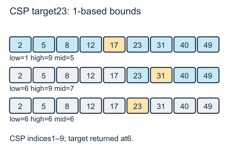Three search ranges use positions 1 through 9 and narrow to target 23 at position 6. This example uses AP-style list positions 1 through 9. Searching for 23 tests the midpoint values 17, 31 and 23 and returns position 6. The list is sorted before searching.

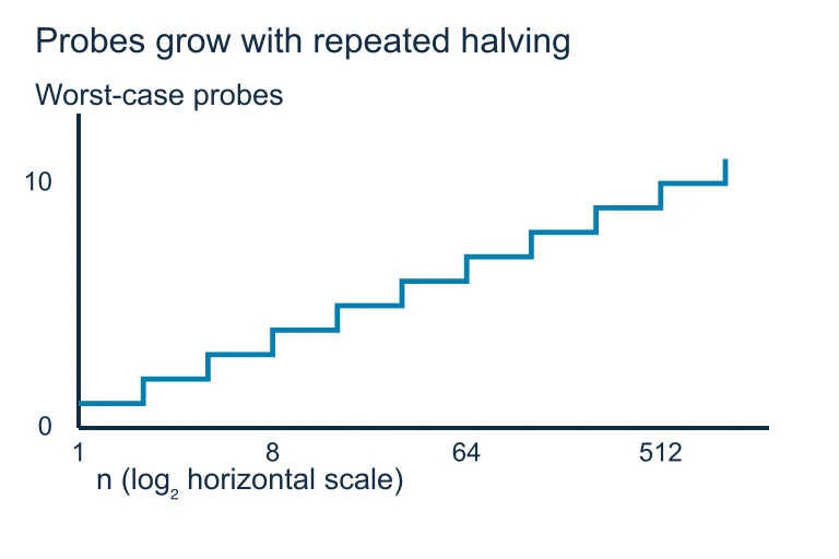A step graph plots the exact worst-case binary-search probe count against list size on a log₂ horizontal axis. For inclusive midpoint binary search on n ≥ 1 items, the maximum number of probes is floor(log₂ n) + 1. The horizontal axis uses a log₂ scale; the count measures search probes after sorting.

SECTION 6

Worked Example — Counting Operations

Let us work through a concrete example of analyzing the efficiency of a simple algorithm. Consider the following procedure that finds the maximum value in a list of n numbers by comparing each element to a running maximum.

ℹ

ALGORITHM — Find Maximum

PROCEDURE FindMax(aList) max ← aList[1] FOR EACH item IN aList IF item > max max ← item RETURN max

Determining the Time Complexity of FindMax

1
Step 1 — Identify the Input Size

The input to this algorithm is aList, a list of n numbers. The input size is therefore n, the number of elements in the list.

n = length of aList
2
Step 2 — Count the Operations in the Loop

The FOR EACH loop iterates over every element in the list. On each iteration, it performs one comparison (item > max) and potentially one assignment (max ← item). In the worst case (when the list is in ascending order), the assignment happens on every iteration. This gives us 2 operations per iteration × n iterations = 2n operations inside the loop.

Loop operations: 2n (worst case)
3
Step 3 — Count Operations Outside the Loop

The initialization max ← aList[1] is 1 operation, and the RETURN max is 1 operation. These are constant operations that do not depend on n.

Outside loop: 2 operations (constant)
4
Step 4 — Combine and Simplify

The total operation count is f(n) = 2n + 2. Applying Big-O simplification rules: drop the constant coefficient 2 and the additive constant 2, since they become negligible as n grows. The dominant term is n.

f(n) = 2n + 2 → O(n) — Linear Time
5
Step 5 — Interpret the Result

The FindMax algorithm runs in linear time. This means that if you double the size of the list, the running time approximately doubles as well. This is a reasonable algorithm—it can handle even very large lists efficiently. In fact, O(n) is the best possible time complexity for finding the maximum of an unsorted list, because any correct algorithm must examine every element at least once.

SECTION 7

Comparing Algorithm Efficiency — Tradeoffs

When choosing between algorithms for the same task, efficiency is the primary consideration, but it is not the only one. Algorithms often involve tradeoffs between time and space, between simplicity and performance, and between worst-case guarantees and typical-case behavior. The table below compares several sorting algorithms to illustrate these tradeoffs.

Algorithm	Best Case	Worst Case	Space	Tradeoff
Selection Sort	`O(n²)`	`O(n²)`	`O(1)`	Simple to implement but always quadratic; minimal extra memory.
Insertion Sort	`O(n)`	`O(n²)`	`O(1)`	Excellent on nearly sorted data; still quadratic worst case.
Merge Sort	`O(n log n)`	`O(n log n)`	`O(n)`	Guaranteed efficient but requires extra memory proportional to n.
Binary Search	`O(1)`	`O(log n)`	`O(1)`	Extremely fast but requires the list to be pre-sorted.
Linear Search	`O(1)`	`O(n)`	`O(1)`	Works on any list (sorted or unsorted) but slower for large inputs.

Common algorithm comparisons showing time-space tradeoffs

✦

KEY TAKEAWAY

Choosing an algorithm is like choosing a vehicle for a cross-country delivery route. A bicycle (simple algorithm) works fine for short distances but becomes impractical across thousands of miles, while a cargo jet (efficient algorithm) has high setup costs—it needs a runway and fuel infrastructure—but covers vast distances quickly. In computing, the 'distance' is your input size, and the 'setup cost' is the algorithm's complexity of implementation or its prerequisite data structure (like needing a sorted list for binary search). Always match your algorithm to the scale of your problem.

SECTION 8

Connections to Decidability & Intractability

The study of algorithmic efficiency naturally connects to deeper questions in theoretical computer science. Beyond asking how fast a problem can be solved, we can ask whether it can be solved at all. An undecidable problem is one for which no algorithm can ever produce a correct answer for all possible inputs—the most famous example being the Halting Problem, which asks whether a given program will eventually stop or run forever. Between decidable and undecidable lies the territory of intractable problems—problems that are technically solvable but require unreasonable (super-polynomial) time.

Category	Description	Example	AP CSP Relevance
Efficient (Tractable)	Solvable in polynomial time. These are considered 'reasonable.'	Sorting, searching, shortest path	You should recognize these as having polynomial Big-O.
Intractable	Solvable but no known polynomial-time algorithm exists. Heuristics or approximations are used.	Traveling Salesman, knapsack problem	Know that some problems have no known efficient solution and require heuristic approaches.
Undecidable	No algorithm can solve it for all inputs. It is provably impossible, not just hard.	Halting Problem	Understand that some problems cannot be solved by any algorithm at all.

Tractable, intractable, and undecidable problems

For the AP CSP exam, the key takeaway is that there exists a spectrum of computational difficulty. At one end are problems with elegant, efficient solutions. In the middle are problems where the best known algorithms require exponential time, prompting the use of heuristic approaches that find good-enough solutions without guaranteeing the optimal one. At the far end are undecidable problems that no computer, no matter how powerful, can solve in general. This hierarchy—tractable, intractable, undecidable—represents one of the deepest insights of computer science and directly informs how software engineers approach real-world system design.

💡

LOOKING AHEAD

In more advanced courses (AP CS A, college algorithms courses), you will learn to formally prove lower bounds on problem complexity, analyze average-case running time, and explore NP-completeness in depth. The intuition you build here—that algorithm choice determines whether a solution is practical—is the foundation for all of that advanced theory.

SECTION 9

Practice Problems

Question 1: CONCEPTUAL

An algorithm has the following operation counts for different input sizes: n = 10 → 100 operations n = 20 → 400 operations n = 50 → 2,500 operations n = 100 → 10,000 operations Which of the following best describes the time complexity of this algorithm?

A. O(n)
B. O(n log n)
C. O(n²)
D. O(2ⁿ)

Show answer (C)

The correct answer is C — O(n²). Observe that 10² = 100, 20² = 400, 50² = 2,500, and 100² = 10,000. The operation count equals n² for every input size given, which is the defining pattern of quadratic growth. Option A (O(n)) is incorrect because linear growth would give 10, 20, 50, 100 operations respectively. Option B (O(n log n)) is incorrect because n log n for n = 100 would be approximately 664, not 10,000. Option D (O(2ⁿ)) is incorrect because 2¹⁰ = 1,024 (not 100), and 2²⁰ = 1,048,576 (not 400)—exponential growth is far more explosive than what we observe.

Question 2: BASIC CALCULATION

A sorted list contains 1,024 elements. What is the maximum number of comparisons a binary search algorithm will make to determine whether a target value is in the list?

A. 10
B. 32
C. 512
D. 1,024

Show answer (A)

The correct answer is A — 10. Binary search halves the remaining search space with each comparison. Starting with 1,024 elements: after 1 comparison → 512, after 2 → 256, after 3 → 128, after 4 → 64, after 5 → 32, after 6 → 16, after 7 → 8, after 8 → 4, after 9 → 2, after 10 → 1. Mathematically, log₂(1,024) = 10. Option B (32) is incorrect; this might result from computing √1,024, which is not how binary search works. Option C (512) is half the list size, which would apply to a linear search on average but not binary search. Option D (1,024) is the worst case for linear search, not binary search.

Question 3: INTERMEDIATE

A programmer is developing a route-finding application and must choose an algorithm for a task where the number of possible solutions grows exponentially with the number of cities. Which TWO of the following statements are true about this situation?

A. A heuristic algorithm can provide an approximate solution in a reasonable amount of time.
B. No computer program can produce any solution to this problem because it is undecidable.
C. The problem can be solved exactly in polynomial time by using binary search.
D. Checking every possible route is impractical for large numbers of cities because the time required grows unreasonably fast.

Show answer (A,D)

The correct answers are A and D. This scenario describes the Traveling Salesman Problem, which has an exponential (or factorial) number of possible routes. Statement A is correct because heuristics—such as nearest-neighbor or genetic algorithms—can find good (though not guaranteed optimal) solutions in polynomial time. Statement D is correct because with n cities, a brute-force approach checks n! routes, which becomes computationally infeasible even for modest n (e.g., 20! ≈ 2.4 × 10¹⁸). Statement B is incorrect because the problem is not undecidable—it is intractable. An exact solution exists and can theoretically be found; it just takes an unreasonable amount of time. Statement C is incorrect because binary search is a searching algorithm for sorted lists and is irrelevant to the combinatorial optimization of routes.

Question 4: APPLIED

3 pts

A social media platform needs to search through user profiles. Currently, profiles are stored in an unsorted list and the platform uses linear search. (a) If the platform has 50,000 profiles, what is the maximum number of profiles that would need to be checked using linear search to find a specific user? (1 point) (b) A developer proposes sorting the profiles and switching to binary search. After sorting, what is the maximum number of profiles that would need to be checked to find a specific user? Show your reasoning. (1 point) (c) Explain one tradeoff the platform must consider when switching from linear search to binary search. (1 point)

Show answer

Rubric: Part (a) — 1 point: Linear search in the worst case checks every element, so the maximum number is 50,000. Award 1 point for stating 50,000 (or n). Part (b) — 1 point: Binary search checks at most ⌈log₂(50,000)⌉ profiles. Since 2¹⁵ = 32,768 and 2¹⁶ = 65,536, the answer is 16 comparisons. Award 1 point for the correct answer of approximately 16 with reasoning that references halving the search space or computing log₂(50,000). Part (c) — 1 point: Award 1 point for identifying a valid tradeoff, such as: the list must be sorted first, which takes O(n log n) time; if new profiles are added frequently, the list must be re-sorted or maintained in sorted order, adding overhead; or sorting requires additional processing time upfront that is only worthwhile if searches are performed frequently.

Question 5: CRITICAL THINKING

4 pts

Consider two algorithms, Algorithm X and Algorithm Y, that both solve the same problem. • Algorithm X runs in O(n) time but uses O(n) additional memory. • Algorithm Y runs in O(n²) time but uses O(1) additional memory. (a) Explain what it means for Algorithm X to use O(n) additional memory and for Algorithm Y to use O(1) additional memory. (1 point) (b) For an input of n = 1,000,000, describe the practical difference in time efficiency between Algorithm X and Algorithm Y. Use specific numbers to support your explanation. (1 point) (c) Describe a scenario in which a programmer might reasonably choose Algorithm Y over Algorithm X, despite Algorithm Y being slower. Justify your reasoning. (1 point) (d) A third algorithm, Algorithm Z, solves the same problem in O(2ⁿ) time. Explain why Algorithm Z would be classified as 'unreasonable' and describe what approach a programmer might use instead if only Algorithm Z could produce an exact solution. (1 point)

Show answer

Rubric: Part (a) — 1 point: O(n) additional memory means Algorithm X requires extra memory that grows proportionally with the input size—for example, it might create a copy of the list or use an auxiliary data structure of size n. O(1) additional memory means Algorithm Y uses a fixed, constant amount of extra memory (e.g., a few variables) regardless of how large the input is. Award 1 point for correctly explaining both. Part (b) — 1 point: For n = 1,000,000, Algorithm X performs on the order of 1,000,000 operations (O(n)), while Algorithm Y performs on the order of 1,000,000² = 1,000,000,000,000 (one trillion) operations (O(n²)). Algorithm Y requires approximately one million times as many operations as Algorithm X. Award 1 point for correctly computing or estimating both values and identifying the dramatic difference. Part (c) — 1 point: A programmer might choose Algorithm Y if the device has very limited memory (such as an embedded system or IoT device) where allocating O(n) extra memory is infeasible, and the input sizes are small enough that O(n²) time is still acceptable. Alternatively, if n is guaranteed to be small, the quadratic time may be negligible while saving memory. Award 1 point for a plausible scenario that correctly identifies memory constraints or small input sizes as the justification. Part (d) — 1 point: Algorithm Z is unreasonable because O(2ⁿ) grows super-polynomially: even for n = 100, 2¹⁰⁰ ≈ 1.27 × 10³⁰ operations, which would take longer than the age of the universe on current hardware. Since Algorithm Z is the only exact solution, a programmer would use a heuristic approach—an algorithm that finds an approximate (good enough) solution in a reasonable (polynomial) amount of time, trading guaranteed optimality for practical feasibility. Award 1 point for correctly explaining why O(2ⁿ) is unreasonable with a concrete example or comparison, and for identifying heuristics as the alternative approach.

SUMMARY

Summary — Algorithmic Efficiency

Summary

Algorithmic efficiency measures how an algorithm's resource consumption—primarily time and space—grows as the input size n increases. We express this growth using Big-O notation, which captures the worst-case upper bound while ignoring constant factors and lower-order terms. Common complexity classes range from O(1) constant through O(log n) logarithmic, O(n) linear, and O(n log n) linearithmic (all reasonable) to O(2ⁿ) exponential and O(n!) factorial (unreasonable).

The distinction between reasonable (polynomial) and unreasonable (super-polynomial) running times is a central concept on the AP CSP exam. When a problem has no known efficient solution, heuristic algorithms provide approximate solutions in reasonable time. Beyond efficiency, some problems are undecidable—no algorithm can solve them for all inputs. Key search algorithms to know are linear search (O(n)) and binary search (O(log n), requires sorted data). Algorithm choice involves tradeoffs between time, space, simplicity, and preconditions—and the best choice depends on the problem's scale and constraints.