Sorting Algorithms - AP Computer Science A

SECTION 1

Historical Context & Motivation

The problem of arranging data into a meaningful order is as old as computing itself. Before electronic computers existed, human "computers" sorted census cards, library catalogs, and financial records by hand—a tedious, error-prone process. When programmable machines emerged in the mid-twentieth century, researchers quickly recognized that sorting was among the most fundamental operations a computer could perform, since so many other tasks—searching, merging, reporting—depend on data being in order. The quest to sort faster and more efficiently has driven some of the most important breakthroughs in algorithm design and analysis.

1945 • John von Neumann's Merge Sort

Von Neumann described the merge sort algorithm in his work on the EDVAC computer, establishing one of the first divide-and-conquer approaches to sorting.

1956 • Bubble Sort Formalized

Researchers formally analyzed simple exchange-based sorting, giving rise to the well-known bubble sort and highlighting the need for more efficient alternatives.

1959 • Shell Sort Introduced

Donald Shell published an improved insertion sort variant that used decreasing gap sequences, demonstrating that clever modifications to simple algorithms could yield significant performance gains.

1962 • Quicksort by Tony Hoare

C.A.R. Hoare introduced quicksort, which became one of the most widely used sorting algorithms in practice due to its excellent average-case performance.

1973 • Big-O Analysis Standardized

Donald Knuth's The Art of Computer Programming rigorously formalized asymptotic notation, giving programmers a universal language to compare sorting algorithm efficiency.

For the AP Computer Science A exam, you need to understand three specific sorting algorithms: selection sort, insertion sort, and merge sort. The central question is not just how each one works mechanically, but why certain approaches are dramatically faster than others as the data set grows—and how to express that difference formally using Big-O notation.

SECTION 2

Core Principles & Definitions

A sorting algorithm is a well-defined sequence of steps that takes a collection of elements—typically an array or ArrayList—and rearranges them into a specified order, most commonly ascending. In Java and on the AP exam, the elements are usually int values or objects that implement the Comparable interface, allowing pairwise comparisons. Every sorting algorithm is built from two primitive operations: comparing two elements to determine their relative order and swapping (or moving) elements to place them in the correct position. The efficiency of a sorting algorithm is measured by how many comparisons and swaps it requires as a function of the input size n.

Comparison-Based Sorting

All three AP-tested algorithms determine order by comparing pairs of elements. The number of comparisons is the primary cost metric. No comparison-based sort can do better than O(n log n) in the general case.

In-Place vs. Out-of-Place

An in-place sort rearranges elements within the original array using O(1) extra memory. Selection sort and insertion sort are in-place; merge sort requires O(n) additional space for its temporary arrays.

Stable vs. Unstable

A stable sort preserves the relative order of equal elements. Insertion sort and merge sort are stable; selection sort is not. Stability matters when sorting objects by multiple keys.

Iterative vs. Recursive

Selection sort and insertion sort use iteration (loops) to process the array. Merge sort uses recursion—dividing the problem into smaller subproblems and combining the results.

Big-O Time Complexity

Big-O notation describes the upper bound on growth rate. Selection and insertion sort are O(n²) in the worst case, while merge sort achieves O(n log n). This difference becomes enormous as n grows.

✦

KEY TAKEAWAY

Think of sorting like organizing a bookshelf. Selection sort is like scanning the entire shelf for the shortest book and placing it first, then scanning the remaining books for the next shortest—simple but slow because you re-scan everything each time. Insertion sort is like picking up books one at a time and sliding each into its correct place among the already-organized ones—fast if the shelf is nearly sorted. Merge sort is like dividing the shelf into halves, sorting each half separately, and then merging the two halves together—a strategy that scales elegantly because the merge step is efficient.

SECTION 3

Visual Explanation

Selection Sort — Step by Step

The following diagram illustrates selection sort operating on the array {5, 3, 8, 1, 4}. In each pass, the algorithm locates the minimum element in the unsorted portion (shown in the right region) and swaps it into the next position of the sorted portion (shown in the left region). The cyan bars represent elements that have been placed in their final sorted position, while the violet bars represent the unsorted elements still being processed.

Selection sort processes the array {5, 3, 8, 1, 4} in four passes. Cyan bars indicate elements locked into their final sorted positions; violet bars remain unsorted. Each pass finds the minimum of the unsorted portion and swaps it to the front.

Notice the key invariant in the diagram: after pass k, the first k elements of the array are in their final sorted positions. The algorithm does not revisit or re-compare sorted elements; it only searches through the remaining unsorted portion. However, the unsorted region only shrinks by one element per pass, which is why the total number of comparisons follows the triangular number pattern: (n − 1) + (n − 2) + ⋯ + 1 = n(n − 1) / 2. This sum grows quadratically, giving selection sort its O(n²) classification.

SECTION 4

How Each Algorithm Works

Selection Sort

Selection sort works by repeatedly selecting the smallest element from the unsorted portion of the array and swapping it into the leftmost unsorted position. For an array of size n, the outer loop runs n − 1 times. On each iteration i, the algorithm scans elements from index i + 1 to n − 1 to find the index of the minimum value, then swaps arr[i] with arr[minIndex]. The inner loop performs n − 1 − i comparisons on pass i. Because the number of comparisons is fixed regardless of the initial ordering, selection sort always runs in exactly O(n²) time in the best, average, and worst cases. It performs at most n − 1 swaps, making it efficient in terms of writes, though this advantage rarely matters in practice.

Insertion Sort

Insertion sort builds a sorted sub-array one element at a time. Starting from index 1, it takes the current element (the "key") and shifts it leftward through the sorted portion until it finds the correct position. In Java, this involves saving arr[j] to a temporary variable, then using a while loop to shift larger elements one position to the right, and finally placing the key in the vacated slot. The critical difference from selection sort is that insertion sort's inner loop can terminate early: if the key is already larger than the element to its left, no shifting is needed. This means that on nearly sorted data, insertion sort approaches O(n) time, while its worst case (reverse-sorted data) remains O(n²).

Merge Sort

Merge sort is a divide-and-conquer algorithm. It recursively splits the array into halves until each sub-array contains a single element (which is trivially sorted), then merges the sorted halves back together. The merge step is the heart of the algorithm: two sorted sub-arrays are combined by comparing their front elements and appending the smaller one to a temporary array, repeating until all elements are merged. This merge operation takes O(n) time for two sub-arrays of total size n. Since the array is split in half at each recursive level and there are log₂ n levels, the total time complexity is O(n log n) in all cases—best, average, and worst. The trade-off is that merge sort requires O(n) additional space for the temporary array used during merging.

SELECTION / INSERTION SORT COMPARISONS

T(n) = n × (n − 1) / 2 → O(n²)

Where n is the number of elements. The sum (n−1) + (n−2) + ⋯ + 1 equals n(n−1)/2, which is proportional to n² for large n.

MERGE SORT RECURRENCE

T(n) = 2 × T(n/2) + O(n) → O(n log n)

Two recursive calls on halves of size n/2, plus O(n) work for the merge step at each level. By the Master Theorem (or by unrolling), this resolves to O(n log₂ n).

SECTION 5

Merge Sort — Detailed Breakdown

Merge sort deserves special attention because it introduces the concept of recursive problem decomposition, which appears throughout computer science. The diagram below traces the complete execution of merge sort on a six-element array, showing the recursive splitting phase (top to bottom) and the merging phase (bottom to top). Understanding this tree-like structure is essential for recognizing why the algorithm achieves O(n log n) performance and why it requires temporary storage.

Merge sort recursively divides {38, 27, 43, 3, 9, 82} into single-element sub-arrays (amber divide phase), then merges them back together in sorted order (green merge phase). Each level performs at most n comparisons, and there are approximately log₂ n levels.

In the divide phase (amber region), the array is halved repeatedly: {38, 27, 43, 3, 9, 82} → {38, 27, 43} and {3, 9, 82} → individual elements. No comparisons occur during splitting; the array is simply partitioned by index. The real work happens in the merge phase (green region), where sorted sub-arrays are combined. When merging {27, 38, 43} with {3, 9, 82}, the algorithm compares 3 < 27 (take 3), 9 < 27 (take 9), 27 < 82 (take 27), 38 < 82 (take 38), 43 < 82 (take 43), then appends 82—a total of five comparisons to merge six elements. This linear merge cost, performed at each of the log₂ n levels, gives the algorithm its characteristic O(n log n) behavior.

💡

AP Exam Tip

On the AP exam, you will not be asked to implement merge sort from scratch. However, you must understand its recursive structure, be able to trace the divide and merge steps on small arrays, and know that it runs in O(n log n) time with O(n) extra space. Free-response questions may ask you to write code that uses the Arrays.sort() or Collections.sort() methods, which internally use variants of merge sort and quicksort.

SECTION 6

Worked Example — Insertion Sort Trace

Let us trace insertion sort on the array {7, 2, 5, 1, 8} step by step, tracking both the comparisons and the element shifts at each pass. This detailed walkthrough demonstrates how the sorted portion grows from left to right and how early termination of the inner loop works.

Insertion Sort on {7, 2, 5, 1, 8}

1
Step 1 — Pass for index 1 (key = 2)

Save key = arr[1] = 2. Compare key with arr[0] = 7. Since 2 < 7, shift 7 one position to the right. No more elements to compare. Insert key at index 0.

Array after pass: {2, 7, 5, 1, 8} — 1 comparison, 1 shift
2
Step 2 — Pass for index 2 (key = 5)

Save key = arr[2] = 5. Compare key with arr[1] = 7. Since 5 < 7, shift 7 right. Compare key with arr[0] = 2. Since 5 ≥ 2, stop. Insert key at index 1.

Array after pass: {2, 5, 7, 1, 8} — 2 comparisons, 1 shift
3
Step 3 — Pass for index 3 (key = 1)

Save key = arr[3] = 1. Compare with 7 → shift; compare with 5 → shift; compare with 2 → shift. No more elements to the left. Insert key at index 0. This is the worst-case scenario for this pass: the key must travel all the way to the front.

Array after pass: {1, 2, 5, 7, 8} — 3 comparisons, 3 shifts
4
Step 4 — Pass for index 4 (key = 8)

Save key = arr[4] = 8. Compare with arr[3] = 7. Since 8 ≥ 7, the inner loop terminates immediately. Key stays in place. This illustrates early termination—no shifts needed when the element is already in the correct relative position.

Final sorted array: {1, 2, 5, 7, 8} — 1 comparison, 0 shifts
5
Step 5 — Totals

Across all four passes: 1 + 2 + 3 + 1 = 7 comparisons and 1 + 1 + 3 + 0 = 5 shifts. For an array of size 5, the worst case would be 4 + 3 + 2 + 1 = 10 comparisons (fully reverse-sorted). The best case would be 4 comparisons with 0 shifts (already sorted). This example falls between the two extremes, reflecting typical behavior.

Total: 7 comparisons, 5 shifts

An archivist holds one portrait card above a gap between four cards on a table. Holding a card aside makes room to shift neighboring cards. In insertion sort, saving the key before shifting protects the value that will be inserted.

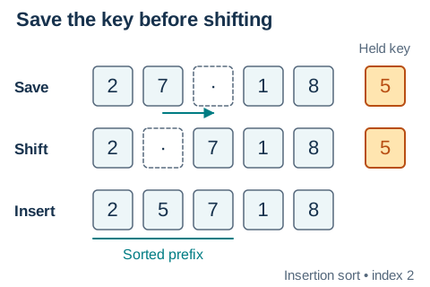Three rows show key 5 held separately, 7 shifted right, and the completed array [2, 5, 7, 1, 8]. The first three entries form the sorted prefix. Starting from [2, 7, 5, 1, 8], save key 5 from index 2, shift 7 right, then insert 5 after 2. The dotted position marks the insertion gap; Java array assignments overwrite values rather than create an empty cell.Open full diagram

SECTION 7

Comparing the Three Algorithms

Choosing the right sorting algorithm depends on context: the size of the data, whether it is partially sorted, how much memory is available, and whether stability matters. The table below provides a comprehensive comparison of the three algorithms tested on the AP Computer Science A exam. Understanding these trade-offs is essential for both the multiple-choice and free-response sections.

Property	Selection Sort	Insertion Sort	Merge Sort
Best-case time	O(n²)	O(n)	O(n log n)
Average-case time	O(n²)	O(n²)	O(n log n)
Worst-case time	O(n²)	O(n²)	O(n log n)
Space complexity	O(1)	O(1)	O(n)
Stable?	No	Yes	Yes
Approach	Iterative	Iterative	Recursive (divide and conquer)
Best suited for	Small arrays; minimal swap cost	Nearly sorted data; small arrays	Large data sets; guaranteed performance

Comparison of AP-tested sorting algorithms

✦

KEY TAKEAWAY

Think of it like mail delivery routes. Selection sort and insertion sort are like a mail carrier who must visit every house on a single long street—the work scales with the square of the number of houses because each trip involves scanning the remaining houses. Merge sort is like dividing the neighborhood among multiple carriers who each sort their own section independently and then combine the results—the parallel structure drastically reduces total effort. For 1,000 elements, O(n²) means roughly 1,000,000 operations while O(n log n) means roughly 10,000—a hundredfold difference that grows even larger as n increases.

SECTION 8

Connection to Advanced Sorting Theory

While the AP Computer Science A exam focuses on selection sort, insertion sort, and merge sort, the broader field of sorting algorithms is rich with alternatives that exploit different data characteristics. Understanding where the AP algorithms sit in this landscape deepens your conceptual understanding and prepares you for college-level data structures courses.

AP-Level Concept	Advanced Extension
Selection sort scans for the minimum each pass	Heap sort uses a binary heap to find the minimum in O(log n) time per extraction, achieving O(n log n) in-place
Insertion sort shifts elements one at a time	Shell sort uses decreasing gap sequences to move elements farther in fewer steps, reducing comparisons substantially
Merge sort divides in half, then merges	Quicksort partitions around a pivot element, achieving O(n log n) average time in-place but O(n²) worst case
All AP sorts are comparison-based: O(n log n) lower bound	Radix sort and counting sort bypass comparisons by exploiting digit/key structure, achieving O(nk) or O(n + k) time
Java's Arrays.sort() and Collections.sort()	Java uses Timsort (a hybrid of merge sort and insertion sort) for objects and dual-pivot quicksort for primitives

AP concepts and their advanced counterparts

A fundamental theorem in computer science, the comparison-based sorting lower bound, proves that any algorithm which sorts by comparing pairs of elements must make at least Ω(n log n) comparisons in the worst case. This means merge sort is asymptotically optimal for comparison-based sorting—no comparison sort can beat O(n log n) in general. When you study data structures in college, you will encounter algorithms that circumvent this bound by using non-comparison techniques, and you will analyze the trade-offs between time, space, stability, and implementation complexity in much greater depth.

SECTION 9

Practice Problems

Question 1: CONCEPTUAL

Which of the following correctly describes a key difference between selection sort and insertion sort?

A. Selection sort is recursive, while insertion sort is iterative.
B. Insertion sort always performs fewer comparisons than selection sort regardless of the initial data order.
C. Insertion sort can terminate its inner loop early when the element is in the correct position, giving it O(n) best-case performance, while selection sort always performs O(n²) comparisons.
D. Selection sort requires O(n) extra space, while insertion sort is in-place.

Show answer (C)

C is correct. Insertion sort's inner loop compares the current key to the element on its left and stops as soon as the key is greater than or equal to that element. When the array is already sorted, each pass requires only one comparison, yielding O(n) total. Selection sort must always scan the entire unsorted portion to find the minimum, regardless of data order, resulting in n(n−1)/2 comparisons every time. A is wrong because both selection sort and insertion sort are iterative. B is wrong because in the worst case (reverse-sorted data), insertion sort also performs O(n²) comparisons—the same as selection sort. D is wrong because both algorithms are in-place, using O(1) additional space.

Question 2: BASIC CALCULATION

Consider the following array:int[] arr = {9, 4, 6, 2, 7};After two complete passes of selection sort (sorting in ascending order), what is the state of the array?

A. {2, 4, 6, 9, 7}
B. {2, 4, 9, 6, 7}
C. {4, 6, 2, 7, 9}
D. {2, 9, 4, 6, 7}

Show answer (A)

A is correct. Pass 1: Scan indices 0–4 for the minimum. The minimum is 2 at index 3. Swap arr[0]=9 with arr[3]=2. Array becomes {2, 4, 6, 9, 7}. Pass 2: Scan indices 1–4 for the minimum. The minimum is 4 at index 1. It is already in place (swap with itself). Array remains {2, 4, 6, 9, 7}. B is wrong because it incorrectly swaps the second minimum into position while leaving 9 at index 2 rather than index 3. C is wrong because it describes passes of a different algorithm (possibly bubble sort). D is wrong because it only performs the first swap correctly and does not complete the second pass properly.

Question 3: INTERMEDIATE

An array of 1,000 elements is already sorted in ascending order. Approximately how many comparisons will insertion sort make, and approximately how many comparisons will merge sort make?

A. Insertion sort: ~999; Merge sort: ~10,000
B. Insertion sort: ~500,000; Merge sort: ~10,000
C. Insertion sort: ~999; Merge sort: ~500,000
D. Insertion sort: ~500,000; Merge sort: ~500,000

Show answer (A)

A is correct. When data is already sorted, insertion sort's inner loop terminates after one comparison per pass (the key is already ≥ the element to its left). Over n − 1 = 999 passes, this yields ~999 comparisons—its O(n) best case. Merge sort does not adapt to sorted input; it always divides and merges all levels. With n = 1,000, it performs approximately 1,000 × log₂(1,000) ≈ 1,000 × 10 = ~10,000 comparisons. B is wrong because 500,000 ≈ n²/2 is the worst-case count for insertion sort, not the best case. C is wrong because merge sort never degrades to O(n²). D is wrong because both values represent worst-case quadratic behavior, which does not apply to either algorithm in this scenario.

Question 4: APPLIED

4 pts

Write a complete Java method public static void selectionSort(int[] arr) that sorts the array in ascending order using the selection sort algorithm. Then, write a second method public static void insertionSort(int[] arr) that sorts the array in ascending order using insertion sort. For each method, clearly use a loop structure that reflects the algorithm's logic.

Show answer

Rubric (4 points): Point 1 — Selection sort outer loop: The method uses an outer for loop that iterates from index 0 to arr.length − 2 (inclusive), representing each position to be filled with the next smallest element. Point 2 — Selection sort inner loop and swap: An inner for loop scans from i + 1 to arr.length − 1, tracking the index of the minimum value. After the inner loop, the element at the minimum index is swapped with arr[i] using a temporary variable.

public static void selectionSort(int[] arr) {
    for (int i = 0; i < arr.length - 1; i++) {
        int minIndex = i;
        for (int j = i + 1; j < arr.length; j++) {
            if (arr[j] < arr[minIndex]) {
                minIndex = j;
            }
        }
        int temp = arr[i];
        arr[i] = arr[minIndex];
        arr[minIndex] = temp;
    }
}

Point 3 — Insertion sort outer loop: The method uses an outer for loop from index 1 to arr.length − 1. On each iteration, it saves the current element as the key (temp variable). Point 4 — Insertion sort inner loop with early termination: A while loop (or equivalent) shifts elements right while they are greater than the key and the index is ≥ 0. The key is then placed in the vacated position. The while loop condition must correctly implement early termination.

public static void insertionSort(int[] arr) {
    for (int i = 1; i < arr.length; i++) {
        int temp = arr[i];
        int j = i - 1;
        while (j >= 0 && arr[j] > temp) {
            arr[j + 1] = arr[j];
            j--;
        }
        arr[j + 1] = temp;
    }
}

Question 5: CRITICAL THINKING

3 pts

A student claims: "Since merge sort is always O(n log n), it is always the best choice for sorting. We should never use selection sort or insertion sort." Evaluate this claim. Describe at least two specific scenarios where selection sort or insertion sort might be preferred over merge sort, and explain why.

Show answer

Rubric (3 points): Point 1 — Nearly sorted data scenario: The student identifies that when data is nearly or already sorted, insertion sort achieves O(n) performance—significantly faster than merge sort's O(n log n). Merge sort does not adapt to the initial ordering and always performs the same number of operations regardless of how sorted the input is. Point 2 — Small array size or memory constraints: The student identifies that for small arrays (e.g., n < 20), the overhead of merge sort's recursive calls and temporary array allocation can make it slower in practice than the simpler loop structure of selection or insertion sort. Additionally, merge sort requires O(n) extra space, which may be problematic in memory-constrained environments. Both selection sort and insertion sort operate in-place with O(1) extra space. Point 3 — Nuanced evaluation of the claim: The student clearly explains that Big-O notation describes asymptotic growth for large n and does not account for constant factors, overhead, or special properties of the input. The student concludes that the claim is overly simplistic: the best algorithm depends on context, including data size, initial ordering, memory availability, and whether stability is required. A complete answer acknowledges that real-world sorting libraries (like Java's Timsort) use hybrid approaches that combine the strengths of multiple algorithms.

SUMMARY

Sorting Algorithms — Key Concepts Review

Summary

The AP Computer Science A exam tests three sorting algorithms. Selection sort repeatedly finds the minimum element in the unsorted portion and swaps it into place, always performing O(n²) comparisons regardless of input order. Insertion sort builds a sorted sub-array by shifting elements to insert each new key in its correct position; its inner loop can terminate early, yielding O(n) best-case performance on nearly sorted data, though its worst case is still O(n²). Both are iterative, in-place algorithms best suited for small data sets.

Merge sort uses a divide-and-conquer strategy—recursively splitting the array in half, sorting each half, and merging the results. It guarantees O(n log n) time in all cases at the cost of O(n) extra space. For the exam, be prepared to trace each algorithm on small arrays, compare their time complexities, identify which is stable or unstable, and recognize when each is most appropriate. Remember that Java's built-in Arrays.sort() and Collections.sort() methods use optimized hybrid algorithms internally, but understanding these three foundational sorts gives you the conceptual toolkit to analyze any sorting scenario.