Representations of Solutions - AP Chemistry

SECTION 1

Historical Context & Motivation

For most of human history, solutions were understood only through their observable properties—taste, color, and conductivity—without any framework for what was happening at the molecular level. The quest to represent what solutions actually look like at the particulate scale drove some of the most consequential advances in chemistry. Understanding the history of how scientists developed representations of solutions reveals the progressive refinement from macroscopic observation to the particulate-level models that anchor modern AP Chemistry.

1803 • Dalton's Atomic Theory

John Dalton proposed that all matter consists of indivisible atoms, providing the first theoretical basis for thinking about dissolved substances as discrete particles rather than continuous fluids.

1884 • Arrhenius Electrolyte Theory

Svante Arrhenius proposed that electrolytes dissociate into ions when dissolved in water, establishing the need for particulate-level diagrams that show separate cations and anions surrounded by solvent molecules.

1923 • Debye–Hückel Theory

Peter Debye and Erich Hückel modeled ionic atmospheres in solution, demonstrating that dissolved ions do not behave independently—they are surrounded by shells of oppositely charged ions and oriented solvent molecules, enriching the way we represent ion-solvent interactions.

1960s • Molecular Modeling & Computation

Advances in computational chemistry allowed scientists to simulate solute–solvent interactions at the molecular level. Ball-and-stick and space-filling models became standard tools for visualizing how solutes are dispersed within a solvent framework.

2010s • AP Chemistry Curriculum Redesign

The College Board restructured AP Chemistry to emphasize particulate-level representations as a core science practice, requiring students to draw and interpret diagrams showing individual atoms, ions, and molecules in solution.

The central question that emerged from this historical arc remains the one you will master in this lesson: How do we accurately represent the composition, structure, and interactions within a solution at both the macroscopic and particulate levels? Answering this question requires fluency in translating between chemical formulas, concentration expressions, and particulate diagrams—skills that are tested repeatedly on the AP Chemistry exam.

SECTION 2

Core Principles & Definitions

A solution is a homogeneous mixture in which one or more solutes are uniformly dispersed within a solvent at the molecular or ionic level. Unlike heterogeneous mixtures—where distinct phases can be identified—solutions exhibit uniform composition throughout, meaning any representative sample drawn from the mixture has the same ratio of solute to solvent particles. The ability to represent this uniformity using particulate diagrams, chemical equations, and concentration expressions forms the foundation of this topic.

Particulate Representations

Diagrams that depict individual atoms, molecules, or ions in solution. Solute particles are shown uniformly dispersed among solvent particles, reflecting the homogeneity of the mixture. Electrolytes are shown as dissociated ions, not intact formula units.

Electrolyte vs. Nonelectrolyte

Strong electrolytes (e.g., NaCl, HCl) fully dissociate into ions and are represented as separated ions. Weak electrolytes (e.g., CH₃COOH) partially ionize, so diagrams show a mixture of molecules and ions. Nonelectrolytes (e.g., C₆H₁₂O₆) remain intact molecules.

Concentration Expressions

Molarity (M), molality (m), mass percent, mole fraction, and parts per million (ppm) all quantify solute–solvent ratios. Particulate diagrams can be used to count particles and directly calculate these values for a given sample.

Solute–Solvent Interactions

Dissolution occurs when solute–solvent intermolecular forces are comparable to or exceed solute–solute and solvent–solvent forces. Representations often show hydration shells around ions or hydrogen bonding between polar solute molecules and water.

Chemical Equations for Dissolution

Dissolution equations represent the process symbolically: NaCl(s) → Na⁺(aq) + Cl⁻(aq). The '(aq)' label indicates the ion is surrounded by water molecules and is a critical part of representing solutions in equation form.

✦

KEY TAKEAWAY

Think of a solution like a crowd at a stadium where every person has been assigned a seat using a random number generator. No matter which section you examine, the ratio of fans wearing home jerseys to those wearing away jerseys is the same. In a particulate diagram of a solution, the solute particles should be uniformly distributed among solvent particles—never clustered in one region. If the solute is a strong electrolyte, each formula unit must be shown as its constituent ions, not as an intact compound.

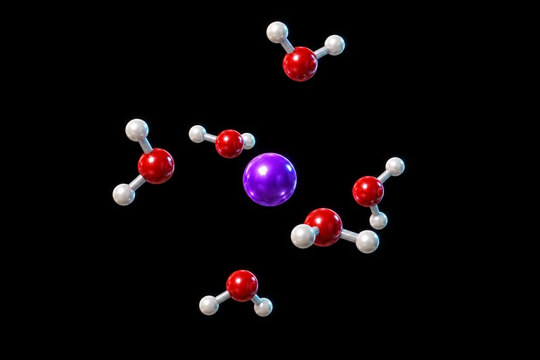Water orientation around one sodium ion Water molecules orient their partially negative oxygen atoms toward a sodium ion.

SECTION 3

Visual Explanation — Particulate Diagrams

The particulate diagram is arguably the most important representational tool tested on the AP Chemistry exam. These diagrams depict a magnified view of a small volume of solution, showing individual particles as circles or clusters of circles. The diagram below contrasts three types of aqueous solutions: a strong electrolyte, a weak electrolyte, and a nonelectrolyte—all at the same overall molar concentration.

The left panel shows NaCl fully dissociated into Na⁺ and Cl⁻ ions—no intact NaCl units remain. The center panel depicts acetic acid, a weak electrolyte, with mostly undissociated CH₃COOH molecules and a small fraction of H⁺ and CH₃COO⁻ ions. The right panel shows glucose, a nonelectrolyte, as intact C₆H₁₂O₆ molecules dispersed among water molecules.

Notice several critical features in the diagram above. First, solute particles are uniformly distributed throughout the solvent in all three panels—this is what distinguishes a solution from a suspension or colloid. Second, the strong electrolyte panel contains no intact NaCl formula units; a common AP exam error is drawing paired Na⁺ and Cl⁻ touching each other. Third, the weak electrolyte panel shows an equilibrium mixture: the dominant species is the intact molecular form, with only a small percentage present as ions. This distinction between strong and weak electrolytes is one of the most frequently tested concepts in the representation of solutions.

SECTION 4

Mathematical Framework — Concentration Expressions

Quantifying the composition of a solution requires expressing the ratio of solute to solvent (or to total solution) using one of several concentration expressions. Each expression has particular utility depending on the context—colligative properties, dilution calculations, or stoichiometric analysis. Particulate diagrams can be connected directly to these expressions by counting the relative number of solute and solvent particles depicted.

MOLARITY

M = n_solute / V_solution

M = molarity (mol·L⁻¹), n_solute = moles of solute, V_solution = volume of solution in liters. Molarity is the most commonly used concentration unit in AP Chemistry and is essential for stoichiometric calculations involving solutions.

DILUTION EQUATION

M₁V₁ = M₂V₂

M₁ and V₁ are the initial molarity and volume; M₂ and V₂ are the final molarity and volume. This equation derives from conservation of moles: the total moles of solute remain constant when solvent is added.

MOLE FRACTION

χ_A = n_A / (n_A + n_B + ···)

χ_A = mole fraction of component A. All mole fractions in a solution sum to 1. This is dimensionless and is used in Raoult's law and colligative property calculations.

MOLALITY

m = n_solute / m_solvent (kg)

m = molality (mol·kg⁻¹). Unlike molarity, molality is independent of temperature because it is defined relative to mass rather than volume. This makes it the preferred unit for colligative property expressions such as boiling-point elevation and freezing-point depression.

💡

AP Exam Tip

When a particulate diagram shows a certain number of solute and solvent particles in a defined volume, you may be asked to calculate the molarity. Count each dissociated ion separately—for example, one formula unit of CaCl₂ produces three ions (one Ca²⁺ and two Cl⁻). However, the molarity of CaCl₂ is based on the original formula units dissolved, not the total number of ions.

SECTION 5

Classifying Solutions by Electrolyte Behavior

A major component of representing solutions accurately is classifying the solute by its electrolyte behavior—that is, its degree of dissociation or ionization in aqueous solution. This classification directly determines what species appear in a particulate diagram and what net ionic equations look like. The table below summarizes the three categories with examples, dissolution equations, and the corresponding particulate features.

Category	Examples	Dissolution Equation	Particulate Diagram Feature
Strong electrolyte	NaCl, KNO₃, HCl, NaOH, CaCl₂	NaCl(s) → Na⁺(aq) + Cl⁻(aq)	Only separated ions; no intact formula units; use → (not ⇌)
Weak electrolyte	CH₃COOH, HF, NH₃, H₂CO₃	CH₃COOH(aq) ⇌ CH₃COO⁻(aq) + H⁺(aq)	Mostly intact molecules with a few ions; use ⇌ to indicate equilibrium
Nonelectrolyte	C₆H₁₂O₆, C₂H₅OH, CO(NH₂)₂	C₆H₁₂O₆(s) → C₆H₁₂O₆(aq)	Only intact molecules; no ions present; does not conduct electricity

Classification of solutes by electrolyte behavior in aqueous solution

This decision flowchart guides you from a dissolved substance to its classification. On the AP exam, you will frequently need to identify whether a solute is a strong electrolyte, weak electrolyte, or nonelectrolyte in order to draw or interpret particulate diagrams correctly.

When drawing particulate diagrams on the AP exam, a critical rule to internalize is the one-to-many principle for strong electrolytes: one formula unit of CaCl₂ produces one Ca²⁺ ion and two Cl⁻ ions, so if you dissolve four formula units, your diagram must show four Ca²⁺ and eight Cl⁻ ions uniformly dispersed. Similarly, one formula unit of Al₂(SO₄)₃ dissociates into two Al³⁺ and three SO₄²⁻ ions. Maintaining the correct stoichiometric ratio of ions is essential for receiving full credit on free-response questions.

SECTION 6

Worked Example — Interpreting a Particulate Diagram

Consider the following scenario: A particulate diagram of a 1.00 L aqueous solution shows 6 Na⁺ ions, 6 Cl⁻ ions, 2 Ca²⁺ ions, and 4 Cl⁻ ions (for a total of 10 Cl⁻ ions), uniformly distributed among water molecules. Each particle in the diagram represents 0.10 mol. Determine the molarity of each dissolved salt and the total Cl⁻ concentration.

Finding Molarities from a Particulate Diagram

1
Step 1 — Identify the Ions and Their Sources

The diagram contains Na⁺, Ca²⁺, and Cl⁻ ions. NaCl dissociates as NaCl → Na⁺ + Cl⁻, so 6 Na⁺ ions correspond to 6 original NaCl formula units. CaCl₂ dissociates as CaCl₂ → Ca²⁺ + 2 Cl⁻, so 2 Ca²⁺ ions correspond to 2 original CaCl₂ formula units, producing 4 Cl⁻ ions. Total Cl⁻ = 6 (from NaCl) + 4 (from CaCl₂) = 10, which matches the diagram.

NaCl: 6 formula units; CaCl₂: 2 formula units
2
Step 2 — Convert Particle Counts to Moles

Each particle represents 0.10 mol, so: moles of NaCl = 6 × 0.10 mol = 0.60 mol and moles of CaCl₂ = 2 × 0.10 mol = 0.20 mol.

n(NaCl) = 0.60 mol; n(CaCl₂) = 0.20 mol
3
Step 3 — Calculate Molarities

M = n / V. For NaCl: M = 0.60 mol / 1.00 L = 0.60 M. For CaCl₂: M = 0.20 mol / 1.00 L = 0.20 M.

M(NaCl) = 0.60 M; M(CaCl₂) = 0.20 M
4
Step 4 — Calculate Total Cl⁻ Concentration

Total Cl⁻ moles = (6 + 4) × 0.10 mol = 1.00 mol. Therefore, [Cl⁻] = 1.00 mol / 1.00 L = 1.00 M. Equivalently, [Cl⁻] = (1)(0.60) + (2)(0.20) = 0.60 + 0.40 = 1.00 M, using the stoichiometric coefficients from each dissociation equation.

[Cl⁻] = 1.00 M

⚠

Common Mistake

Students often confuse the molarity of the dissolved compound with the concentration of an individual ion. The molarity of CaCl₂ is 0.20 M, but the concentration of Cl⁻ contributed by CaCl₂ alone is 0.40 M because each formula unit releases two chloride ions. Always apply the stoichiometric coefficient from the dissociation equation.

SECTION 7

Comparing Representation Types

AP Chemistry expects you to move fluidly between three levels of representation: the macroscopic (what you observe), the particulate (molecular-level diagrams), and the symbolic (chemical equations, formulas, and concentration expressions). Each representation has distinct strengths and limitations for communicating solution properties. The table below compares these three levels.

Feature	Macroscopic	Particulate	Symbolic
What it shows	Observable properties: color, phase, conductivity	Individual atoms, molecules, and ions in relative positions	Chemical formulas, equations, concentration values
Strengths	Directly observable; intuitive; connects to lab experience	Shows degree of dissociation; reveals molecular interactions; distinguishes strong from weak electrolytes	Compact; allows quantitative calculations; universally standardized
Limitations	Cannot distinguish between electrolyte types; no molecular detail	Not to scale; limited particle count represents a vast number of actual molecules	Abstract; does not convey spatial arrangement or relative proportions visually
AP exam usage	Lab-based questions; identifying solution properties	Drawing or interpreting diagrams (very common on FRQs)	Balancing equations; stoichiometry; concentration calculations

Comparison of macroscopic, particulate, and symbolic representations of solutions

✦

KEY TAKEAWAY

Think of these three representation levels as three languages that describe the same reality—like a photograph (macroscopic), an architectural blueprint (particulate), and the building specifications spreadsheet (symbolic). An expert chemist, like an expert architect, moves seamlessly between all three. The AP exam specifically tests your ability to translate between representations: given a particulate diagram, write the dissolution equation; given a formula, draw the correct particulate diagram; given macroscopic observations, identify the particulate-level explanation.

SECTION 8

Connections to Advanced Topics

The representations of solutions you have studied here form the conceptual scaffolding for several more advanced AP Chemistry topics. Understanding how to depict dissolved species accurately is not an isolated skill—it connects directly to equilibrium expressions, acid-base theory, electrochemistry, and colligative properties. Recognizing these connections now will help you see the bigger picture of the AP Chemistry curriculum.

This Lesson's Concept	Advanced Extension	How They Connect
Strong vs. weak electrolyte diagrams	Equilibrium & acid-base chemistry	Weak electrolyte diagrams show equilibrium mixtures; the ratio of ions to molecules relates to Ka or Kb values
Ion concentration calculations	Solubility equilibria (Ksp)	Ksp expressions require knowing the concentrations of individual dissociated ions—directly from particulate-level thinking
Molarity and dilution	Solution stoichiometry & titrations	Titration calculations rely on M₁V₁ = M₂V₂ and on correctly identifying species in solution
Number of dissolved particles	Colligative properties	Boiling-point elevation and freezing-point depression depend on the total number of dissolved particles (van 't Hoff factor i), not just moles of solute
Ion identification in solution	Electrochemistry & galvanic cells	Half-cell reactions require knowing which ions are present in the electrolyte solution, informed by dissociation representations

How representations of solutions connect to later AP Chemistry topics

One particularly important forward connection is the van 't Hoff factor (i), which quantifies how many particles a single formula unit produces upon dissolution. For NaCl, i = 2; for CaCl₂, i = 3; for glucose, i = 1. This factor appears directly in colligative property equations like ΔT_b = i × K_b × m. The ability to determine i comes directly from the particulate representations studied in this lesson—if you can draw the correct diagram, you can count the particles and determine i.

SECTION 9

Practice Problems

Question 1: CONCEPTUAL

A particulate diagram of an aqueous solution shows only intact molecules uniformly distributed among water molecules. No separated ions are present. Which of the following solutes could produce this diagram?

A. NaCl
B. HCl
C. C₆H₁₂O₆ (glucose)
D. KOH

Show answer (C)

The correct answer is C. Glucose (C₆H₁₂O₆) is a nonelectrolyte—it dissolves as intact molecules without producing any ions. This is consistent with a diagram showing only molecules and no ions. NaCl (A) is a strong electrolyte that would fully dissociate into Na⁺ and Cl⁻ ions, so the diagram would show separated ions, not intact formula units. HCl (B) is a strong acid and strong electrolyte in water, fully dissociating into H⁺ and Cl⁻; no intact HCl molecules would remain. KOH (D) is a strong base and strong electrolyte, producing K⁺ and OH⁻ ions upon dissolution.

Question 2: BASIC CALCULATION

A 500.0 mL aqueous solution contains 0.30 mol of dissolved CaCl₂. What is the molar concentration of Cl⁻ ions in the solution?

A. 0.30 M
B. 0.60 M
C. 1.20 M
D. 1.80 M

Show answer (C)

The correct answer is C. CaCl₂ is a strong electrolyte: CaCl₂(s) → Ca²⁺(aq) + 2 Cl⁻(aq). Each mole of CaCl₂ produces 2 moles of Cl⁻, so 0.30 mol CaCl₂ yields 0.60 mol Cl⁻. The molarity of Cl⁻ = 0.60 mol / 0.5000 L = 1.20 M. Option A (0.30 M) incorrectly uses the moles of CaCl₂ without the stoichiometric factor or volume conversion. Option B (0.60 M) applies the stoichiometric factor but uses the wrong volume (1.00 L instead of 0.500 L). Option D (1.80 M) incorrectly assumes three Cl⁻ ions per formula unit, perhaps confusing CaCl₂ with a trivalent salt.

Question 3: INTERMEDIATE

A particulate diagram of an aqueous weak acid HA shows 12 intact HA molecules and 3 A⁻ ions (along with 3 H⁺ ions) in a volume representing 0.500 L. If each particle in the diagram represents 0.020 mol, what is the percent ionization of HA and the molarity of HA at equilibrium?

A. Percent ionization = 20%; [HA] = 0.48 M
B. Percent ionization = 25%; [HA] = 0.48 M
C. Percent ionization = 20%; [HA] = 0.60 M
D. Percent ionization = 25%; [HA] = 0.36 M

Show answer (A)

The correct answer is A. The total initial HA = 12 intact + 3 ionized = 15 formula units. Percent ionization = (3/15) × 100% = 20%. The equilibrium concentration of HA: 12 particles × 0.020 mol/particle = 0.24 mol; [HA] = 0.24 mol / 0.500 L = 0.48 M. Option B uses 3/12 = 25%, incorrectly dividing ionized particles by remaining HA rather than the total initial amount. Option C calculates percent ionization correctly but uses the total initial moles (0.30 mol / 0.500 L = 0.60 M) instead of the equilibrium HA moles. Option D combines both errors.

Question 4: APPLIED

10 pts

A student dissolves three different solutes—NaCl, CaCl₂, and C₆H₁₂O₆—each at a concentration of 0.10 M, in separate 1.00 L beakers of water. The student then measures the freezing-point depression of each solution. (a) Draw a particulate-level diagram for each solution showing the relative number and types of dissolved species for a sample containing 5 formula units of each solute. Clearly label all species. (b) Rank the three solutions in order of increasing freezing-point depression. Justify your ranking using the van 't Hoff factor. (c) If the measured freezing-point depression of the NaCl solution is 0.348 °C and Kf for water is 1.86 °C·kg/mol, calculate the experimental van 't Hoff factor for NaCl. Comment on whether this value is consistent with expectations. (d) The student claims that if both NaCl and CaCl₂ were dissolved in the same beaker at 0.10 M each, the total Cl⁻ concentration would be 0.30 M. Evaluate this claim.

Show answer

Point-by-point rubric: (a) Particulate diagrams (3 points): • 1 point: NaCl diagram shows 5 Na⁺ and 5 Cl⁻ ions uniformly distributed, with no intact NaCl units. • 1 point: CaCl₂ diagram shows 5 Ca²⁺ and 10 Cl⁻ ions uniformly distributed, with no intact CaCl₂ units. • 1 point: C₆H₁₂O₆ diagram shows 5 intact glucose molecules uniformly distributed, with no ions. (b) Ranking and justification (3 points): • 1 point: Correct ranking: C₆H₁₂O₆ < NaCl < CaCl₂. • 1 point: Identifying the van 't Hoff factors: i = 1 for glucose, i = 2 for NaCl, i = 3 for CaCl₂. • 1 point: Explaining that ΔTf = i × Kf × m, so higher i at the same molality produces greater freezing-point depression. (c) Calculating experimental i (2 points): • 1 point: Correct setup: ΔTf = i × Kf × m → 0.348 = i × 1.86 × 0.10 → i = 0.348 / 0.186 = 1.87. • 1 point: Noting that the theoretical i for NaCl is 2.00, and the experimental value of 1.87 is slightly less due to ion pairing (interionic attractions in solution reduce the effective number of independent particles). This is consistent with expectations. (d) Evaluating the claim (2 points): • 1 point: NaCl contributes 1 × 0.10 M = 0.10 M Cl⁻; CaCl₂ contributes 2 × 0.10 M = 0.20 M Cl⁻. • 1 point: Total [Cl⁻] = 0.10 + 0.20 = 0.30 M. The student's claim is correct.

Question 5: CRITICAL THINKING

10 pts

A researcher prepares four aqueous solutions and measures their electrical conductivity. The data are shown below. Solution A: 0.10 M HCl — Conductivity: High Solution B: 0.10 M CH₃COOH — Conductivity: Low Solution C: 0.10 M NaOH — Conductivity: High Solution D: 0.10 M C₂H₅OH (ethanol) — Conductivity: None (a) For each solution, classify the solute as a strong electrolyte, weak electrolyte, or nonelectrolyte. Justify each classification using the conductivity data. (b) Draw particulate-level diagrams for Solutions B and D, clearly showing the relative proportions of molecular and ionic species. Explain the key differences between the two diagrams. (c) Solutions A and B are mixed in equal volumes. Using Le Chatelier's principle, predict qualitatively what happens to the equilibrium position of acetic acid ionization. Support your prediction with a net ionic equation. (d) A student proposes that if Solution D were replaced with 0.10 M sucrose (C₁₂H₂₂O₁₁), the conductivity result would be the same. Evaluate this claim and explain the underlying chemical reasoning.

Show answer

Point-by-point rubric: (a) Classification (4 points): • 1 point: HCl is a strong electrolyte because it fully dissociates into H⁺ and Cl⁻, producing high conductivity. • 1 point: CH₃COOH is a weak electrolyte because it partially ionizes, producing few ions and hence low conductivity. • 1 point: NaOH is a strong electrolyte because it fully dissociates into Na⁺ and OH⁻, producing high conductivity. • 1 point: C₂H₅OH is a nonelectrolyte because it dissolves as intact molecules without producing any ions, resulting in zero conductivity. (b) Particulate diagrams (3 points): • 1 point: Solution B diagram shows mostly intact CH₃COOH molecules with a few H⁺ and CH₃COO⁻ ions, all uniformly distributed among water molecules. • 1 point: Solution D diagram shows only intact C₂H₅OH molecules uniformly distributed among water molecules with no ions present. • 1 point: The key difference is that Solution B contains some ions (reflecting partial ionization of the weak acid), while Solution D contains no ions at all. Both show intact molecules, but only B has an equilibrium between molecular and ionic forms. (c) Mixing analysis (2 points): • 1 point: When HCl (a source of H⁺) is added to the acetic acid equilibrium CH₃COOH ⇌ CH₃COO⁻ + H⁺, Le Chatelier's principle predicts the equilibrium shifts to the left (toward reactants) because the concentration of H⁺ has been increased. The net ionic equation for the reaction is: H⁺(aq) + CH₃COO⁻(aq) → CH₃COOH(aq). • 1 point: This means the proportion of undissociated CH₃COOH molecules in the particulate diagram would increase, and the number of acetate and hydrogen ions would decrease relative to the original Solution B. (d) Sucrose evaluation (1 point): • 1 point: The claim is correct. Sucrose is also a nonelectrolyte (a molecular compound that does not ionize in water), so it would dissolve as intact C₁₂H₂₂O₁₁ molecules and produce zero conductivity, just like ethanol. The underlying reason is the same: neither compound produces ions in solution because neither undergoes dissociation or ionization; both interact with water through intermolecular forces (hydrogen bonding) without breaking covalent bonds.

SUMMARY

Lesson Summary

Summary

Representing solutions in AP Chemistry requires fluency in three interconnected levels: macroscopic observations (color, conductivity, phase), particulate diagrams (showing individual atoms, molecules, and ions uniformly distributed in solvent), and symbolic representations (chemical equations, formulas, and concentration expressions like molarity, molality, and mole fraction). The defining feature of any solution is its homogeneity—solute particles must be uniformly dispersed in every diagram you draw.

The electrolyte classification of the solute determines the correct particulate representation: strong electrolytes appear as fully dissociated ions with no intact formula units; weak electrolytes show an equilibrium mixture of mostly intact molecules with a small fraction of ions; and nonelectrolytes appear only as intact molecules. When calculating ion concentrations from these diagrams, always apply the stoichiometric coefficients from the dissolution equation—a skill that connects directly to the van 't Hoff factor, colligative properties, equilibrium, and electrochemistry in later units.