Properties of Photons - AP Chemistry

SECTION 1

Historical Context & Motivation

Classical physics treated light as a continuous wave—an electromagnetic disturbance described perfectly by Maxwell's equations, capable of diffraction, interference, and polarization. Yet by the close of the nineteenth century, several experimental puzzles resisted any wave-only interpretation. The spectrum of radiation emitted by a heated blackbody diverged catastrophically from classical predictions at short wavelengths, a failure dubbed the ultraviolet catastrophe. Simultaneously, the photoelectric effect—the ejection of electrons from a metal surface by light—produced results that no wave model could explain: increasing intensity increased the number of emitted electrons but not their kinetic energy, while light below a threshold frequency ejected no electrons regardless of brightness.

1900 • Planck's Quantum Hypothesis

Max Planck resolved the ultraviolet catastrophe by proposing that energy is emitted and absorbed in discrete packets of size E = hν, introducing the fundamental constant h.

1905 • Einstein's Photon Model

Albert Einstein extended Planck's idea, asserting that light itself consists of quantized particles—photons—each carrying energy hν. This explained the photoelectric effect and earned him the 1921 Nobel Prize.

1913 • Bohr's Atomic Model

Niels Bohr applied quantized photon emission and absorption to hydrogen, predicting discrete spectral lines that matched experimental data with remarkable precision.

1923 • Compton Scattering

Arthur Compton demonstrated that X-ray photons scatter off electrons with a change in wavelength, confirming photon momentum and solidifying the particle nature of light.

These discoveries opened a central question for chemistry: if light comes in discrete packets whose energy depends on frequency alone, how do photons interact with atoms and molecules to produce the characteristic emission and absorption spectra that form the basis of spectroscopy? Understanding the properties of photons is therefore essential for interpreting atomic structure, electronic transitions, and the analytical techniques that rely on them.

SECTION 2

Core Principles & Definitions

A photon is the quantum of electromagnetic radiation—the smallest indivisible unit of light energy. Unlike classical particles, a photon has zero rest mass and always travels at the speed of light c ≈ 3.00 × 10⁸ m s⁻¹ in vacuum. Its energy is determined exclusively by its frequency (or equivalently, its wavelength), linking the wave and particle descriptions of electromagnetic radiation through a set of foundational relationships.

Quantized Energy

Photon energy is E = hν. Higher frequency means more energy per photon; this is not adjustable by changing amplitude or intensity.

Wave–Particle Duality

Photons exhibit both wave properties (interference, diffraction) and particle properties (discrete absorption, momentum transfer). The experiment determines which aspect is observed.

Speed & Rest Mass

All photons travel at c = 3.00 × 10⁸ m s⁻¹ in vacuum with zero rest mass, regardless of frequency or energy.

Inverse Wavelength–Frequency Relationship

Since c = λν, a photon's wavelength and frequency are inversely proportional: short-wavelength photons (UV, X-ray) are high-energy; long-wavelength photons (IR, radio) are low-energy.

Photon Momentum

Despite zero rest mass, photons carry momentum p = h/λ, confirmed by Compton scattering—important for understanding radiation pressure and photon–electron interactions.

SECTION 3

Visual Explanation — The Electromagnetic Spectrum & Photon Energy

The electromagnetic spectrum arranged from high-energy, short-wavelength UV at left to low-energy, long-wavelength IR at right. The three boxed equations—E = hν, c = λν, and p = h/λ—link a photon's wave description to its particle properties. Notice how UV photons carry roughly five times the energy of IR photons.

The diagram above encapsulates the essential quantitative relationships governing photon behavior. Moving leftward along the spectrum, wavelength decreases while frequency and energy per photon increase. This inverse relationship is not merely academic: it dictates which photons have sufficient energy to excite electronic transitions in atoms (typically UV and visible), which excite molecular vibrations (infrared), and which are too low in energy to interact with most chemical bonds (microwave and radio). In AP Chemistry, you will most often encounter photons in the context of atomic emission and absorption spectra, where the photon energy must exactly match the energy gap between two quantized electronic states.

SECTION 4

Mathematical Framework

Three interrelated equations form the mathematical backbone of photon physics as applied in AP Chemistry. Mastering these relationships—and knowing when to combine them—is critical for solving problems involving electromagnetic radiation, spectral analysis, and the photoelectric effect.

PLANCK–EINSTEIN RELATION

E = hν

E = energy of one photon (J); h = Planck's constant = 6.626 × 10⁻³⁴ J·s; ν (nu) = frequency of the radiation (Hz = s⁻¹). Energy scales linearly with frequency—doubling ν doubles E.

WAVE EQUATION

c = λν → ν = c/λ → λ = c/ν

c = speed of light = 3.00 × 10⁸ m s⁻¹; λ (lambda) = wavelength (m); ν = frequency (s⁻¹). This equation links wavelength and frequency; since c is constant in vacuum, λ and ν are inversely proportional.

COMBINED PHOTON ENERGY–WAVELENGTH

E = hc/λ

Substituting ν = c/λ into the Planck–Einstein relation yields this highly useful form. Because wavelength is often the experimentally measured quantity (e.g., from a spectrometer), this expression lets you calculate photon energy directly from λ. The product hc ≈ 1.99 × 10⁻²⁵ J·m is a convenient constant to memorize.

ENERGY OF A MOLE OF PHOTONS

E_mol = N_A × hν = N_A × hc/λ

N_A = Avogadro's number = 6.022 × 10²³ mol⁻¹. Multiplying single-photon energy by N_A converts to kJ mol⁻¹, a scale directly comparable to bond energies and reaction enthalpies.

ℹ

Unit Watch

SECTION 5

Photons and Atomic Spectral Lines

The most chemically significant application of photon properties is the production and interpretation of atomic emission and absorption spectra. When an electron in an atom transitions from a higher energy level to a lower one, the atom emits a photon whose energy precisely equals the energy difference between those two levels: ΔE = E_upper − E_lower = hν. Conversely, an atom can absorb a photon only if its energy exactly matches an available transition. Because electronic energy levels are quantized, each element produces a unique set of spectral lines—its spectral fingerprint.

Hydrogen energy level diagram showing three representative transitions. Downward arrows represent photon emission; the photon's wavelength (and color) depend on the magnitude of ΔE between levels. Lyman series transitions terminate at n = 1 and produce UV photons; Balmer series transitions terminate at n = 2 and produce visible-light photons.

The diagram illustrates a crucial principle: the spacing between energy levels converges as n increases, meaning higher-level transitions involve smaller ΔE values and thus longer-wavelength photons. For instance, the n = 3 → n = 2 transition in hydrogen emits a red photon at 656.3 nm, while the n = 2 → n = 1 transition emits a far more energetic UV photon at 121.6 nm. On the AP exam, you may be given an energy level diagram and asked to identify which transition corresponds to a photon of a specified wavelength—or vice versa. The key strategy is always to compute ΔE and then relate it to λ via E = hc/λ.

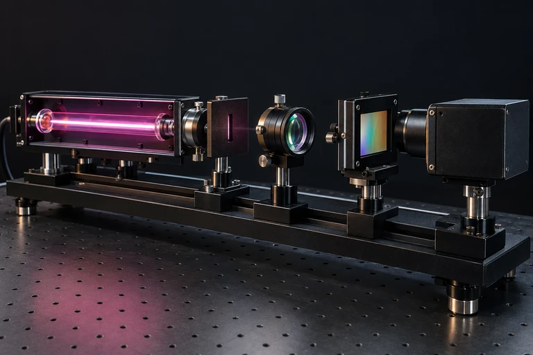Hydrogen discharge tube and spectrometer Light from a hydrogen discharge tube enters a spectrometer, where its component wavelengths can be separated.

SECTION 6

Worked Example

Worked example

1
Step 1 — State the Problem

A photon is emitted when the electron in a hydrogen atom transitions from n = 4 to n = 2. Calculate (a) the energy of the emitted photon in joules, (b) its wavelength in nanometers, and (c) the energy per mole of these photons in kJ mol⁻¹.
2
Step 2 — Find ΔE Using Energy Levels

For hydrogen, E_n = −2.18 × 10⁻¹⁸ J / n². Calculate each level: E₄ = −2.18 × 10⁻¹⁸ / 16 = −1.363 × 10⁻¹⁹ J; E₂ = −2.18 × 10⁻¹⁸ / 4 = −5.450 × 10⁻¹⁹ J. The energy difference: ΔE = E₂ − E₄ = (−5.450 × 10⁻¹⁹) − (−1.363 × 10⁻¹⁹) = −4.087 × 10⁻¹⁹ J. The negative sign indicates energy is released (emission).

E_photon = 4.09 × 10⁻¹⁹ J
3
Step 3 — Calculate Wavelength

Using E = hc/λ, rearrange to λ = hc/E. Substitute: λ = (6.626 × 10⁻³⁴ J·s)(3.00 × 10⁸ m s⁻¹) / (4.087 × 10⁻¹⁹ J) = 4.864 × 10⁻⁷ m. Convert to nm: 4.864 × 10⁻⁷ m × (10⁹ nm/m) = 486.4 nm.

λ = 486 nm (blue-green visible light — Balmer β line)
4
Step 4 — Convert to kJ per Mole

E_mol = N_A × E = (6.022 × 10²³ mol⁻¹)(4.087 × 10⁻¹⁹ J) = 2.461 × 10⁵ J mol⁻¹ = 246 kJ mol⁻¹. This is comparable to the strength of a C–C single bond (~347 kJ mol⁻¹), illustrating that visible-light photons carry energies on the scale of chemical bonds.

E = 246 kJ mol⁻¹

SECTION 7

Applications, Strengths & Limitations

The photon model is indispensable in chemistry, but its application has both powerful strengths and important boundaries. The table below summarizes where the photon model excels and where more advanced treatments become necessary.

Application / Feature	Strength	Limitation
Atomic emission/absorption spectra	Accurately predicts line positions for H-like species; E = hν directly links spectral data to energy gaps	Multi-electron atoms require electron–electron repulsion corrections beyond simple photon energy matching
Photoelectric effect	Explains threshold frequency, independence of KE from intensity, and instantaneous ejection	Does not address electron wave behavior or band structure in metals
Spectroscopy (UV-Vis, IR)	Photon energy matching explains selective absorption; Beer–Lambert law quantifies amount	Selection rules and transition probabilities require quantum mechanical wave functions
Photochemistry	One photon absorbed per molecule per excitation event (Stark–Einstein law)	Multi-photon processes and laser chemistry require advanced photon statistics

Strengths and limitations of the photon model in chemical contexts

SECTION 8

Connection to Advanced Theory

The photon properties you have studied—quantized energy, zero rest mass, wave–particle duality—form the gateway to more advanced quantum mechanical treatments. In general chemistry, we treat photons primarily through the Planck–Einstein relation and apply it to atomic spectra and spectroscopy. In more rigorous courses, these ideas deepen considerably.

Concept in AP Chemistry	Advanced Treatment
E = hν (photon energy)	Quantum electrodynamics (QED) describes photon creation/annihilation operators and vacuum fluctuations
Discrete spectral lines	Schrödinger equation solutions give exact wave functions; selection rules (Δl = ±1) govern which transitions emit/absorb photons
Photoelectric effect (threshold ν)	Solid-state band theory explains work functions; Fermi levels determine electron availability
Beer–Lambert absorption	Transition dipole moment integrals quantify oscillator strength; relates to molar absorptivity ε

AP Chemistry treatment vs. advanced quantum theory

For the AP exam, remember that the photon model seamlessly connects to PES (photoelectron spectroscopy), where high-energy photons ionize core and valence electrons, and the kinetic energies of ejected electrons reveal orbital energy levels. This is a direct extension of Einstein's photoelectric equation: KE = hν − Φ, where Φ is the binding energy of the electron. Understanding photon properties therefore provides the conceptual foundation for interpreting PES data, which is a frequently tested topic.

SECTION 9

Practice Problems

Question 1: CONCEPTUAL

A beam of red light and a beam of violet light have equal intensities (energy per unit time). Which statement correctly compares the two beams?

A. The red beam contains fewer photons per second, each with greater energy.
B. The violet beam contains fewer photons per second, each with greater energy.
C. Both beams contain the same number of photons per second with the same energy per photon.
D. The red beam has higher frequency photons because red light travels faster.

Show answer (B)

B is correct. Violet light has a shorter wavelength and thus higher frequency, so E = hν gives a larger energy per violet photon. Since both beams deliver the same total energy per second, the violet beam must contain fewer photons per second to compensate. A is wrong because red photons have lower energy (lower frequency), not greater. C is wrong because equal intensity does not require equal photon count when photon energies differ. D is wrong because all photons travel at the same speed c regardless of frequency.

Question 2: BASIC CALCULATION

What is the energy of a single photon of light with wavelength 450 nm? (h = 6.626 × 10⁻³⁴ J·s; c = 3.00 × 10⁸ m s⁻¹)

A. 2.98 × 10⁻²⁵ J
B. 4.42 × 10⁻¹⁹ J
C. 1.47 × 10⁻¹⁸ J
D. 6.63 × 10⁻³⁴ J

Show answer (B)

Using E = hc/λ: E = (6.626 × 10⁻³⁴)(3.00 × 10⁸) / (450 × 10⁻⁹) = 1.988 × 10⁻²⁵ / 4.50 × 10⁻⁷ = 4.42 × 10⁻¹⁹ J. B is correct. A (2.98 × 10⁻²⁵ J) is the numerator hc without dividing by λ properly—likely a powers-of-ten error. C (1.47 × 10⁻¹⁸ J) results from failing to convert nm to m (dividing by 450 instead of 4.50 × 10⁻⁷). D is simply Planck's constant itself, not an energy calculation.

Question 3: INTERMEDIATE

An electron in a hydrogen atom transitions from n = 5 to n = 2, emitting a photon. Which transition in the same atom would produce a photon with a longer wavelength?

A. n = 6 → n = 2
B. n = 5 → n = 1
C. n = 4 → n = 2
D. n = 3 → n = 2

Show answer (D)

Longer wavelength means lower photon energy, which requires a smaller ΔE between levels. D (n = 3 → 2) has the smallest energy gap among the choices because the initial level is closest to n = 2. The n = 5 → 2 transition (given) has ΔE = E₂ − E₅, which is larger than ΔE for n = 3 → 2. A (n = 6 → 2) has an even larger ΔE than n = 5 → 2, producing a shorter wavelength. B (n = 5 → 1) terminates at n = 1, which involves a much larger total ΔE. C (n = 4 → 2) has a larger ΔE than n = 3 → 2. Only D yields a smaller energy gap and therefore a longer wavelength.

Question 4: APPLIED

A chemistry student uses a spectrometer and observes that a sample of gaseous sodium absorbs light strongly at 589 nm (the sodium D-line). The student has Planck's constant (h = 6.626 × 10⁻³⁴ J·s), the speed of light (c = 3.00 × 10⁸ m s⁻¹), and Avogadro's number (

N_A

= 6.022 × 10²³ mol⁻¹). (a) Calculate the frequency of the absorbed photon. (b) Calculate the energy of one absorbed photon in joules. (c) Calculate the energy per mole of these photons in kJ mol⁻¹. (d) A student claims that doubling the intensity of the 589 nm light doubles the energy of each absorbed photon. Is this claim correct? Justify your answer in terms of photon properties.

Show answer

(a) ν = c/λ = (3.00 × 10⁸ m s⁻¹)/(5.89 × 10⁻⁷ m) = 5.09 × 10¹⁴ Hz. (b) E = hν = (6.626 × 10⁻³⁴ J·s)(5.09 × 10¹⁴ s⁻¹) = 3.37 × 10⁻¹⁹ J. (c) E_mol = (6.022 × 10²³ mol⁻¹)(3.37 × 10⁻¹⁹ J) = 2.03 × 10⁵ J mol⁻¹ = 203 kJ mol⁻¹. (d) The claim is incorrect. A photon's energy is determined solely by its frequency via E = hν. Doubling the intensity of 589 nm light means doubling the number of photons striking the sample per second, but each photon still has the same energy of 3.37 × 10⁻¹⁹ J. Intensity affects photon flux, not individual photon energy.

Question 5: CRITICAL THINKING

A student measures the wavelengths of photons emitted by a hydrogen discharge tube and collects the following data for four visible emission lines (Balmer series): Line 1: λ = 656.3 nm Line 2: λ = 486.1 nm Line 3: λ = 434.0 nm Line 4: λ = 410.2 nm (a) Calculate the photon energy in joules for Line 1 and Line 4. (b) All four lines belong to the Balmer series (transitions ending at n = 2). Identify the initial quantum number n for Line 1 and Line 4, given that

E_n

= −2.18 × 10⁻¹⁸ / n² J for hydrogen. (c) Using the data, explain the trend in wavelength spacing as the initial quantum number increases. What physical principle accounts for this convergence? (d) Predict what would happen to the Balmer series if the student could observe lines corresponding to transitions from very high n values (n → ∞ to n = 2). State the limiting wavelength and justify your answer.

Show answer

(a) Line 1: E = hc/λ = (1.99 × 10⁻²⁵ J·m)/(6.563 × 10⁻⁷ m) = 3.03 × 10⁻¹⁹ J. Line 4: E = (1.99 × 10⁻²⁵)/(4.102 × 10⁻⁷) = 4.85 × 10⁻¹⁹ J. (b) For Line 1: E_upper = E₂ + ΔE = −5.45 × 10⁻¹⁹ + 3.03 × 10⁻¹⁹ = −2.42 × 10⁻¹⁹ J; solving −2.18 × 10⁻¹⁸/n² = −2.42 × 10⁻¹⁹ gives n² ≈ 9, so n = 3. For Line 4: E_upper = −5.45 × 10⁻¹⁹ + 4.85 × 10⁻¹⁹ = −6.0 × 10⁻²⁰ J; n² ≈ 36, so n = 6. (c) The spacing between successive Balmer lines decreases as n increases because hydrogen's energy levels follow a 1/n² pattern that converges toward zero. The differences between adjacent levels shrink rapidly at high n, causing the emitted photon energies—and therefore wavelengths—to crowd together. (d) When n → ∞,

E_n

approaches 0 J, making ΔE = 0 − (−5.45 × 10⁻¹⁹) = 5.45 × 10⁻¹⁹ J. The series limit wavelength is λ = hc/ΔE = 1.99 × 10⁻²⁵ / 5.45 × 10⁻¹⁹ = 365 nm, in the near-UV region. All Balmer lines converge toward but never exceed this limit.