Introduction to Solubility Equilibria - AP Chemistry

SECTION 1

Historical Context & Motivation

The question of why some salts dissolve readily in water while others remain stubbornly insoluble has fascinated chemists for centuries. Early alchemists and apothecaries catalogued the behaviors of mineral salts long before any theoretical framework existed to explain them. The development of solubility equilibria as a quantitative concept arose from the broader revolution in chemical thermodynamics and equilibrium theory during the nineteenth and early twentieth centuries. Understanding solubility at the molecular level became essential not only for analytical chemistry—where selective precipitation is a cornerstone technique—but also for geology, environmental science, and medicine, where the dissolution and formation of mineral precipitates governs everything from cave formation to kidney stone pathology.

1864 • Law of Mass Action

Cato Guldberg and Peter Waage formulated the law of mass action, establishing that the rate of a chemical reaction is proportional to the product of the concentrations of the reactants raised to appropriate powers. This laid the mathematical groundwork for all equilibrium expressions, including those governing solubility.

1884 • Le Châtelier's Principle

Henri Le Châtelier articulated his principle of dynamic equilibrium, explaining how systems at equilibrium respond to external perturbations. This concept became essential for predicting how changes in ion concentration, temperature, or pH shift solubility equilibria.

1889 • Nernst & Ionic Theory

Walther Nernst, building on Arrhenius's theory of electrolytic dissociation, developed quantitative treatments of ionic equilibria in solution. His work enabled the first rigorous descriptions of how sparingly soluble salts dissociate into their component ions.

1923 • Debye–Hückel Theory

Peter Debye and Erich Hückel published their theory of interionic interactions, introducing activity coefficients that account for nonideal behavior in electrolyte solutions. This refinement was critical for accurate Ksp measurements in solutions of appreciable ionic strength.

With these theoretical tools in hand, chemists could finally answer the central question that motivates this lesson: given any sparingly soluble ionic compound in contact with water, how do we quantitatively predict the concentrations of dissolved ions at equilibrium, and how do we determine whether a precipitate will form when two solutions are mixed? The answer lies in the solubility-product constant, K_sp.

SECTION 2

Core Principles & Definitions

Solubility equilibria describe the dynamic balance that exists when a sparingly soluble ionic solid is in contact with a saturated solution of its ions. At this point, the rate of dissolution equals the rate of precipitation, producing a system where the concentrations of dissolved ions remain constant over time. Unlike the simple solubility rules you may have memorized ("all nitrates are soluble"), the K_sp framework assigns a precise numerical value to the extent of dissolution for any ionic compound. This quantitative approach is fundamental to AP Chemistry because it bridges stoichiometry, equilibrium, and thermodynamics into a single, unified analytical tool.

Solubility-Product Constant (Ksp)

The equilibrium constant for the dissolution of a sparingly soluble salt into its constituent ions. It equals the product of the ion concentrations, each raised to the power of its stoichiometric coefficient. A smaller K_sp indicates lower solubility.

Molar Solubility (s)

The number of moles of solute that dissolve per liter of saturated solution (mol/L). Molar solubility is the quantity you calculate from K_sp using an ICE table. It directly connects the equilibrium expression to measurable solution concentrations.

Ion Product (Q)

The reaction quotient for the dissolution process evaluated at non-equilibrium conditions. Comparing Q to K_sp predicts the system's direction: if Q > K_sp, precipitation occurs; if Q < K_sp, the solution is unsaturated.

Common Ion Effect

The decrease in solubility of a sparingly soluble salt when a soluble salt containing a common ion is added to the solution. This is a direct application of Le Châtelier's principle: increasing one product ion shifts equilibrium back toward the solid.

✦

KEY TAKEAWAY

Think of a saturated solution as a crowded dance floor at capacity. People leave (precipitate) and enter (dissolve) at equal rates, so the number of dancers (dissolved ions) stays constant. K_sp tells you the capacity of the floor—a small K_sp means the room is tiny and only a few dancers can fit. The ion product Q is the current headcount: if Q exceeds the capacity K_sp, people must leave (a precipitate forms).

SECTION 3

Visual Explanation — Dissolution Equilibrium

The diagram shows a saturated AgCl solution at dynamic equilibrium. Ag⁺ ions (purple) and Cl⁻ ions (cyan) populate the solution while the solid sits at the bottom. The green dashed arrow represents dissolution; the red dashed arrow represents precipitation. At equilibrium, both processes occur at equal rates, keeping the ion concentrations constant.

Notice that the equilibrium expression for a dissolution reaction does not include the solid phase—its activity is defined as 1 and is absorbed into the equilibrium constant. For the general dissolution of a salt M_aX_b(s) → aM^b+(aq) + bX^a−(aq), the K_sp expression involves only the aqueous ion concentrations. The solid may vary in amount without affecting the equilibrium, as long as some solid remains present—an essential condition for the K_sp expression to be valid.

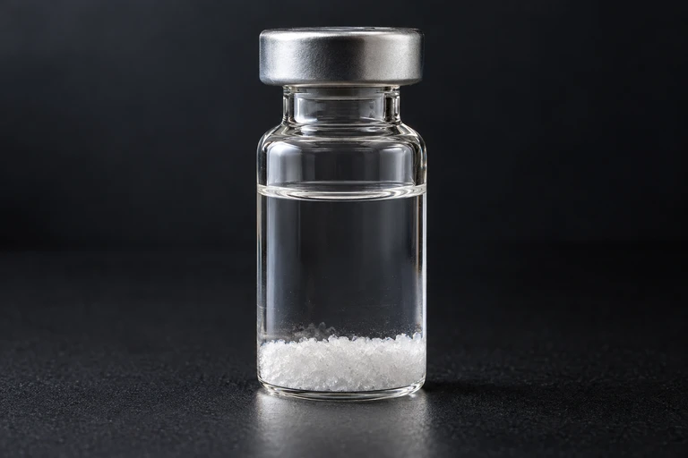Solid and saturated solution in contact A saturated solution can remain in contact with undissolved solid while dissolution and crystallization continue.

SECTION 4

Mathematical Framework

The mathematical treatment of solubility equilibria parallels the general equilibrium framework you already know, with the simplification that the solid phase has unit activity. Let us develop the key equations systematically, beginning with the generic dissolution reaction and building toward the connection between K_sp and molar solubility.

GENERAL DISSOLUTION REACTION

MₐXᵦ(s) ⇌ aM^(b+)(aq) + bX^(a−)(aq)

M represents the cation, X the anion, and a, b are their respective stoichiometric coefficients. The charges on the ions are determined by the requirement for electrical neutrality.

SOLUBILITY-PRODUCT EXPRESSION

Ksp = [M^(b+)]^a × [X^(a−)]^b

The solid's activity is 1 and does not appear. Each concentration is raised to the power of its stoichiometric coefficient. This expression is valid only when excess solid is present.

MOLAR SOLUBILITY (1:1 SALT, e.g., AgCl)

Ksp = s × s = s² → s = √Ksp

For a 1:1 salt MX, if s moles dissolve per liter, then [M⁺] = s and [X⁻] = s. This gives the simplest relationship between K_sp and molar solubility.

MOLAR SOLUBILITY (1:2 SALT, e.g., CaF₂)

CaF₂(s) ⇌ Ca²⁺(aq) + 2F⁻(aq) → Ksp = (s)(2s)² = 4s³ → s = ³√(Ksp/4)

If s mol/L of CaF₂ dissolves, then [Ca²⁺] = s and [F⁻] = 2s. The factor of 4 arises from the squared stoichiometric coefficient. This pattern generalizes: for M_aX_b, K_sp = aᵃ × bᵇ × $s^{a+b}$ .

⚠

AP Exam Tip

You cannot directly compare K_sp values to rank solubility unless the salts produce the same total number of ions in the same ratio. A salt with a larger K_sp is not necessarily more soluble than one with a smaller K_sp if the stoichiometries differ. Always convert to molar solubility first when ranking.

SECTION 5

Predicting Precipitation — Q vs. Ksp

One of the most powerful applications of solubility equilibria is predicting whether a precipitate will form when two solutions are mixed. This analysis uses the ion product Q, which has the same mathematical form as the K_sp expression but is evaluated using the actual (possibly non-equilibrium) ion concentrations after mixing. Comparing Q to K_sp tells you definitively whether the solution is unsaturated, saturated, or supersaturated, and therefore whether precipitation will occur. Remember that when you mix two solutions, dilution changes the concentrations—you must calculate the new concentrations in the total mixed volume before computing Q.

This decision diagram summarizes the three possible outcomes when comparing the ion product Q with K_sp. When Q < Ksp, the solution can accommodate more dissolved ions. When Q > Ksp, the solution is supersaturated and a precipitate will form. When Q = Ksp, the system is at equilibrium.

A common procedural error on the AP exam is forgetting to account for the dilution that occurs when two solutions are mixed. If you combine 50.0 mL of 0.010 M AgNO₃ with 50.0 mL of 0.010 M NaCl, the total volume is 100.0 mL, and each ion concentration is halved to 0.0050 M before you compute Q. Only after this dilution correction should you compare Q = (0.0050)(0.0050) = 2.5 × 10⁻⁵ against K_sp for AgCl (1.77 × 10⁻¹⁰). Since Q >> K_sp, AgCl precipitates.

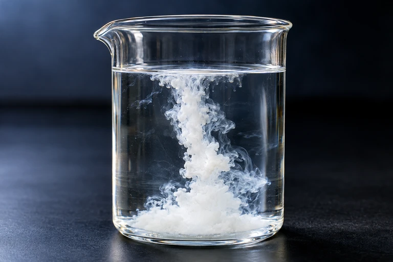Silver chloride precipitation context Silver chloride forms a white precipitate when the dissolved ion product exceeds its solubility product.

SECTION 6

Worked Example — Molar Solubility of PbI₂

Lead(II) iodide is a sparingly soluble salt that produces the iconic yellow precipitate in qualitative analysis. Its dissolution provides an excellent example of a 1:2 stoichiometry problem. Given that K_sp for PbI₂ = 9.8 × 10⁻⁹ at 25 °C, calculate the molar solubility of PbI₂ in pure water.

Molar Solubility of PbI₂

1
Step 1 — Write the Dissolution Equation

PbI₂(s) ⇌ Pb²⁺(aq) + 2I⁻(aq). Identify the stoichiometric ratio: for every mole of PbI₂ that dissolves, one mole of Pb²⁺ and two moles of I⁻ are produced.
2
Step 2 — Set Up the ICE Table

Let s = molar solubility (mol/L of PbI₂ that dissolves). Initial concentrations in pure water: [Pb²⁺] = 0, [I⁻] = 0. Change: [Pb²⁺] increases by +s, [I⁻] increases by +2s. Equilibrium: [Pb²⁺] = s, [I⁻] = 2s.
3
Step 3 — Write the Ksp Expression

K_sp = [Pb²⁺][I⁻]² = (s)(2s)² = (s)(4s²) = 4s³. This is the critical algebraic step—the coefficient 2 in front of I⁻ yields a factor of 4 when squared.
4
Step 4 — Solve for s

Substitute K_sp = 9.8 × 10⁻⁹ into 4s³ = 9.8 × 10⁻⁹. Divide both sides by 4: s³ = 2.45 × 10⁻⁹. Take the cube root: s = (2.45 × 10⁻⁹)^1/3.

s = 1.35 × 10⁻³ mol/L
5
Step 5 — Find Ion Concentrations

[Pb²⁺] = s = 1.35 × 10⁻³ M. [I⁻] = 2s = 2.70 × 10⁻³ M. You can verify by substituting back: K_sp = (1.35 × 10⁻³)(2.70 × 10⁻³)² = (1.35 × 10⁻³)(7.29 × 10⁻⁶) = 9.8 × 10⁻⁹ ✓

[Pb²⁺] = 1.35 × 10⁻³ M, [I⁻] = 2.70 × 10⁻³ M

SECTION 7

Factors Affecting Solubility & Model Limitations

The simple K_sp model is extraordinarily useful but rests on several simplifying assumptions. Understanding both the factors that genuinely shift solubility equilibria and the limitations of the model ensures that you apply it correctly on the AP exam and recognize when more sophisticated treatments are necessary.

Factor	Effect on Solubility	Explanation
Common Ion Effect	Decreases solubility	Adding a common ion increases Q, shifting equilibrium toward solid. Example: Adding NaCl decreases AgCl solubility.
pH Effects	Increases solubility of salts with basic anions	Lowering pH protonates basic anions (e.g., F⁻, CO₃²⁻, OH⁻), removing them from solution and pulling equilibrium toward dissolution.
Temperature	Usually increases solubility	Most dissolution reactions are endothermic, so increasing T favors products (Le Châtelier). Ksp values are temperature-dependent.
Complex Ion Formation	Increases solubility	Ligands (e.g., NH₃, CN⁻) bind metal cations, reducing free [M⁺] and shifting dissolution equilibrium to the right.

Factors that affect solubility equilibria beyond the basic Ksp model

⚠️

MODEL LIMITATIONS

The K_sp model assumes ideal solution behavior—that ion activities equal their molar concentrations. This is reasonable for very dilute solutions of sparingly soluble salts, but in solutions of higher ionic strength, interionic attractions cause effective concentrations (activities) to deviate from measured molarities. The Debye–Hückel theory introduces activity coefficients to correct for this, but such corrections are beyond the scope of the AP exam. Just be aware that K_sp values reported in tables are thermodynamic constants at 25 °C and may not perfectly predict solubility under all real-world conditions.

SECTION 8

Connection to Advanced Equilibrium Concepts

Solubility equilibria do not exist in isolation—they are one facet of the broader equilibrium landscape in chemistry. On the AP exam, you will encounter problems that couple K_sp with other equilibrium constants, particularly the formation constant K_f for complex ion equilibria and K_a/K_b for acid-base equilibria. When two equilibria are coupled, the overall equilibrium constant is the product of the individual constants, reflecting the thermodynamic principle that ΔG° values are additive.

Concept	Basic Ksp Model	Advanced Extension
Equilibrium Constant	Single Ksp for dissolution	Coupled Ksp × Kf for dissolution + complexation; overall K = Ksp × Kf
Ion Interactions	Activities ≈ concentrations (ideal dilute solution)	Activity coefficients from Debye–Hückel theory correct for interionic effects
pH Dependence	Qualitative—"acidic solutions dissolve basic salts"	Quantitative—conditional solubility calculated using Ka to find fraction of anion protonated
Thermodynamic Basis	Ksp as empirical constant	ΔG° = −RT ln Ksp connects solubility to enthalpy and entropy of dissolution

How the Ksp model connects to more advanced equilibrium treatments

A classic example of coupled equilibria is the dissolution of AgCl in ammonia solution. The K_sp for AgCl alone is 1.77 × 10⁻¹⁰, but in concentrated NH₃ the Ag⁺ ions form the complex [Ag(NH₃)₂]⁺ with K_f = 1.7 × 10⁷. The overall reaction AgCl(s) + 2NH₃(aq) ⇌ [Ag(NH₃)₂]⁺(aq) + Cl⁻(aq) has K_overall = K_sp × K_f ≈ 3.0 × 10⁻³, dramatically increasing solubility. This coupling of equilibria illustrates why understanding K_sp in isolation is necessary but not always sufficient for predicting solubility in real chemical systems.

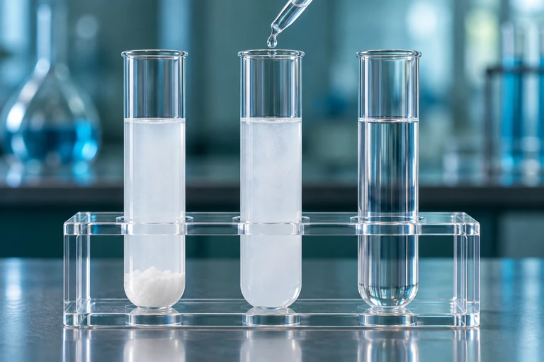Three matched tubes show white suspension, ammonia addition and clear colorless solution; the exact panel shows two-ligand silver complex formation. With sufficient ammonia, AgCl can dissolve as silver forms [Ag(NH₃)₂]⁺. The solubility product uses free Ag⁺ concentration, while total dissolved silver includes both free and complexed silver.

Clear solution still contains silver. With sufficient ammonia, AgCl can dissolve as silver forms [Ag(NH₃)₂]⁺. The solubility product uses free Ag⁺ concentration, while total dissolved silver includes both free and complexed silver. 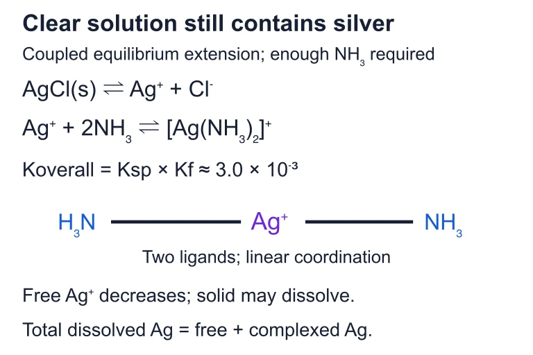With sufficient ammonia, AgCl can dissolve as silver forms [Ag(NH₃)₂]⁺. The solubility product uses free Ag⁺ concentration, while total dissolved silver includes both free and complexed silver.

SECTION 9

Practice Problems

Question 1: CONCEPTUAL

A saturated solution of BaSO₄ is at equilibrium with excess solid BaSO₄. If additional solid BaSO₄ is added to the beaker, what happens to the concentration of Ba²⁺ ions in solution?

A. The concentration of Ba²⁺ increases because more solid is available to dissolve.
B. The concentration of Ba²⁺ decreases because the added solid shifts the equilibrium to the left.
C. The concentration of Ba²⁺ remains unchanged because the solution is already saturated and the activity of a pure solid is constant.
D. The concentration of Ba²⁺ increases temporarily and then returns to its original value.

Show answer (C)

The correct answer is C. The activity of a pure solid is 1 regardless of the amount present, so adding more solid does not change the Ksp expression or the equilibrium ion concentrations. The solution was already saturated, meaning [Ba²⁺] and [SO₄²⁻] were at their equilibrium values. Choice A is incorrect because the solution is already at maximum capacity—additional solid simply remains undissolved. Choice B is incorrect because the solid does not appear in the Ksp expression; its presence cannot shift the equilibrium to the left. Choice D is incorrect because there is no driving force to temporarily increase [Ba²⁺]; the system was at equilibrium before and after the addition.

Question 2: BASIC CALCULATION

The Ksp of AgBr is 5.0 × 10⁻¹³ at 25 °C. What is the molar solubility of AgBr in pure water?

A. 2.5 × 10⁻¹³ M
B. 7.1 × 10⁻⁷ M
C. 5.0 × 10⁻⁷ M
D. 2.2 × 10⁻⁴ M

Show answer (B)

The correct answer is B. AgBr is a 1:1 salt: AgBr(s) ⇌ Ag⁺(aq) + Br⁻(aq). If s = molar solubility, then Ksp = s² = 5.0 × 10⁻¹³. Solving: s = √(5.0 × 10⁻¹³) = 7.1 × 10⁻⁷ M. Choice A incorrectly divides Ksp by 2, treating it like a concentration rather than a product. Choice C takes the square root incorrectly (√5.0 ≈ 2.24, not 1.0). Choice D would correspond to a Ksp of approximately 4.8 × 10⁻⁸, which is far too large and likely results from an exponent error.

Question 3: INTERMEDIATE

The Ksp of Ca(OH)₂ is 4.68 × 10⁻⁶. What is the molar solubility of Ca(OH)₂ in a solution that already contains 0.10 M NaOH?

A. 1.06 × 10⁻² M
B. 4.68 × 10⁻⁴ M
C. 4.68 × 10⁻⁵ M
D. 2.34 × 10⁻³ M

Show answer (B)

The correct answer is B. Ca(OH)₂(s) ⇌ Ca²⁺(aq) + 2OH⁻(aq), so Ksp = [Ca²⁺][OH⁻]². The NaOH provides a common ion: initial [OH⁻] = 0.10 M. Let s = molar solubility. Then [Ca²⁺] = s and [OH⁻] = 0.10 + 2s ≈ 0.10 M (since s << 0.10). Therefore Ksp = s(0.10)² = s(0.010) = 4.68 × 10⁻⁶, giving s = 4.68 × 10⁻⁴ M. Choice A (1.06 × 10⁻²) is the molar solubility in pure water without the common ion, calculated from 4s³ = 4.68 × 10⁻⁶. Choice C divides Ksp by 0.10 instead of (0.10)². Choice D divides Ksp by 2 × 10⁻³, reflecting an error in applying the stoichiometric coefficient.

Question 4: APPLIED

4 pts

A water treatment plant wants to remove fluoride ions from groundwater by adding CaCl₂ to precipitate CaF₂. The groundwater contains [F⁻] = 4.0 × 10⁻³ M. The Ksp of CaF₂ is 3.45 × 10⁻¹¹. (a) Write the balanced dissolution equation for CaF₂ and the corresponding Ksp expression. (b) Calculate the minimum concentration of Ca²⁺ that must be present to initiate precipitation of CaF₂. (c) If 100. mL of 0.20 M CaCl₂ is added to 400. mL of the groundwater, determine the ion product Q and state whether a precipitate forms. (d) Explain how the pH of the groundwater might affect the efficiency of this fluoride removal process.

Show answer

Rubric (4 points): (a) [1 point] CaF₂(s) ⇌ Ca²⁺(aq) + 2F⁻(aq); Ksp = [Ca²⁺][F⁻]². One point for correct balanced equation AND correct Ksp expression. (b) [1 point] For precipitation to begin, Q must equal Ksp. Ksp = [Ca²⁺][F⁻]² → 3.45 × 10⁻¹¹ = [Ca²⁺](4.0 × 10⁻³)² = [Ca²⁺](1.6 × 10⁻⁵). Solving: [Ca²⁺] = 3.45 × 10⁻¹¹ / 1.6 × 10⁻⁵ = 2.2 × 10⁻⁶ M. One point for correct setup and answer. (c) [1 point] After mixing, total volume = 500. mL. [Ca²⁺] = (0.100 L × 0.20 M) / 0.500 L = 0.040 M. [F⁻] = (0.400 L × 4.0 × 10⁻³ M) / 0.500 L = 3.2 × 10⁻³ M. Q = (0.040)(3.2 × 10⁻³)² = (0.040)(1.024 × 10⁻⁵) = 4.1 × 10⁻⁷. Since Q = 4.1 × 10⁻⁷ >> Ksp = 3.45 × 10⁻¹¹, a precipitate does form. One point for correct dilution calculations, correct Q, and correct prediction. (d) [1 point] If the pH of the groundwater is low (acidic conditions), H⁺ ions will react with F⁻ to form HF (Ka = 6.8 × 10⁻⁴, so F⁻ is a weak base). This decreases [F⁻] in solution, which lowers Q and makes precipitation less favorable. Therefore, acidic groundwater reduces the efficiency of fluoride removal because less F⁻ is available to precipitate as CaF₂. One point for correctly identifying that low pH reduces [F⁻] and explaining the impact on precipitation.

Question 5: CRITICAL THINKING

4 pts

A student performs an experiment to determine the Ksp of PbCl₂ by measuring its molar solubility at various temperatures. The data are shown below: Temperature (°C) | Molar Solubility s (mol/L) 20 | 0.036 30 | 0.042 40 | 0.050 50 | 0.059 60 | 0.070 (a) Write the dissolution equation and the Ksp expression for PbCl₂. (b) Calculate Ksp at 20 °C using the student's data. (c) Using the trend in the data, determine whether the dissolution of PbCl₂ is endothermic or exothermic. Justify your answer using Le Châtelier's principle. (d) At 40 °C, a student prepares a solution by dissolving PbCl₂ in 0.10 M HCl. Explain qualitatively, referencing the common ion effect, why the molar solubility of PbCl₂ in this solution would be less than 0.050 mol/L.

Show answer

Rubric (4 points): (a) [1 point] PbCl₂(s) ⇌ Pb²⁺(aq) + 2Cl⁻(aq); Ksp = [Pb²⁺][Cl⁻]². One point for balanced equation and correct expression. (b) [1 point] At 20 °C, s = 0.036 M. [Pb²⁺] = s = 0.036 M and [Cl⁻] = 2s = 0.072 M. Ksp = (0.036)(0.072)² = (0.036)(5.184 × 10⁻³) = 1.9 × 10⁻⁴. One point for correct substitution using proper stoichiometry and correct numerical answer (accept 1.8–1.9 × 10⁻⁴). (c) [1 point] The data show that molar solubility increases with increasing temperature. Since dissolution shifts further toward products at higher temperatures, the equilibrium favors the endothermic direction when heat is added. By Le Châtelier's principle, if increasing temperature shifts the equilibrium to the right (more dissolution), then the forward reaction (dissolution) must be endothermic (ΔH > 0). One point for correct identification as endothermic WITH a valid Le Châtelier justification linking increasing T to the favored direction. (d) [1 point] The 0.10 M HCl provides Cl⁻ ions (HCl is a strong acid that fully dissociates), which is a common ion with the Cl⁻ produced by PbCl₂ dissolution. By Le Châtelier's principle, the increased [Cl⁻] from HCl shifts the dissolution equilibrium to the left, toward the solid. This means less PbCl₂ dissolves, so the molar solubility is reduced below the value in pure water. Mathematically, Ksp = [Pb²⁺](0.10 + 2s)², and since 0.10 >> 2s, the effective [Cl⁻] is much larger, forcing [Pb²⁺] (and thus s) to be much smaller. One point for correctly identifying Cl⁻ as the common ion, applying Le Châtelier's principle, and concluding that solubility decreases.

SUMMARY

Summary & Key Concepts

Summary

Solubility equilibria describe the dynamic balance between a sparingly soluble ionic solid and its dissolved ions in a saturated solution. The solubility-product constant Ksp quantifies this equilibrium as the product of ion concentrations, each raised to its stoichiometric coefficient. The molar solubility (s) can be calculated from K_sp using an ICE table, but the algebraic relationship depends on the stoichiometry of the salt (e.g., K_sp = s² for 1:1 salts versus K_sp = 4s³ for 1:2 salts).

To predict precipitation, compare the ion product Q to K_sp: if Q > K_sp, a precipitate forms; if Q < K_sp, more solid can dissolve. Key factors that modify solubility include the common ion effect (which decreases solubility), pH changes (which increase solubility for salts with basic anions), and complex ion formation (which dramatically increases solubility by removing the free cation from solution). Mastering these relationships is essential for the AP Chemistry exam, where you will encounter both quantitative K_sp calculations and qualitative reasoning about how perturbations shift solubility equilibria.