Common-Ion Effect - AP Chemistry

SECTION 1

Historical Context & Motivation

The story of the common-ion effect is inseparable from the broader history of chemical equilibrium. During the nineteenth century, chemists struggled to explain why the extent of a reaction could change when a seemingly inert substance was added to a solution. Early observations noted that adding table salt to a saturated solution of silver chloride caused additional precipitate to form, a phenomenon that defied the intuitive expectation that an already-saturated solution should remain unchanged. These empirical curiosities pushed researchers toward a quantitative framework for equilibrium that would eventually unify solubility, acid–base chemistry, and buffer design under a single theoretical umbrella.

1864 • Law of Mass Action

Cato Guldberg and Peter Waage formulate the law of mass action, establishing that the rate of a reaction is proportional to the product of the concentrations of the reactants, each raised to a power. This relationship lays the conceptual groundwork for equilibrium constants.

1884 • Le Châtelier's Principle

Henry Louis Le Châtelier publishes his principle stating that a system at equilibrium, when subjected to a stress, will shift to partially counteract that stress. This qualitative rule becomes the conceptual backbone for understanding the common-ion effect.

1889 • Arrhenius Acid–Base Theory

Svante Arrhenius proposes that acids dissociate to produce H⁺ ions and bases produce OH⁻ ions in aqueous solution. His framework allows chemists to explain how adding a strong acid to a weak acid solution suppresses ionization—a direct manifestation of the common-ion effect.

1899 • Walther Nernst & Solubility Product

Walther Nernst formalizes the solubility product constant (Ksp) for sparingly soluble salts. By expressing dissolution equilibria quantitatively, Nernst provides the mathematical tool needed to predict exactly how a common ion reduces solubility.

1916 • Buffer Theory Matures

Lawrence Joseph Henderson's work on carbonate buffers in blood plasma, later formalized by Karl Albert Hasselbalch, demonstrates that buffer capacity depends directly on the common-ion effect: a conjugate pair suppresses excessive ionization and stabilizes pH.

By the early twentieth century, the common-ion effect was recognized not as an isolated curiosity but as a direct consequence of equilibrium dynamics. The central question it addresses is straightforward yet powerful: how does the presence of an ion that already participates in an equilibrium shift the position of that equilibrium? Answering this question quantitatively remains essential for AP Chemistry students who must master solubility equilibria, acid–base buffers, and selective precipitation.

SECTION 2

Core Principles & Definitions

The common-ion effect describes the observation that the solubility of a sparingly soluble salt decreases, or the degree of ionization of a weak electrolyte diminishes, when a solution already contains one of the ions produced by the dissolving or ionizing substance. At its core, this phenomenon is a specific application of Le Châtelier's principle: adding a product ion to an equilibrium system drives the reaction in the reverse direction. To reason about the effect quantitatively, you need to connect equilibrium expressions—K_sp for dissolution, K_a or K_b for acid–base ionization—with the initial concentrations that include the common ion.

Common Ion

An ion that is present in a solution from more than one source. For example, Cl⁻ supplied by both NaCl and PbCl₂ in the same solution.

Equilibrium Shift (Le Châtelier)

Adding a common ion increases Q (the reaction quotient) relative to K, so the system shifts toward reactants to re-establish equilibrium—reducing solubility or suppressing ionization.

Ksp and Solubility

The solubility product constant Ksp is fixed at a given temperature. When a common ion is present, the molar solubility s must decrease so that the ion-product expression still equals Ksp.

Ka/Kb and Ionization

For weak acids or bases, the presence of a common ion (e.g., the conjugate base from an added salt) suppresses ionization, lowering the percent ionization and stabilizing pH—this is the basis of buffer chemistry.

✦

KEY TAKEAWAY

Think of the common-ion effect like a crowded room analogy applied to molecules. Imagine a dance floor (the solution) where couples form spontaneously (dissolution). If you flood the room with extra dance partners of one type (the common ion), fewer new couples form—because the equilibrium between paired and unpaired dancers shifts toward the paired state. The equilibrium constant (the 'social norm' for how many couples exist) doesn't change, but the number of new couples that can spontaneously form decreases.

SECTION 3

Visual Explanation

This bar chart compares the molar solubility of PbCl₂ (K_sp = 1.7 × 10⁻⁵) in pure water versus solutions containing increasing concentrations of NaCl, which supplies the common ion Cl⁻. Notice how the solubility drops dramatically as [Cl⁻] increases.

The diagram above illustrates the quantitative impact of the common-ion effect on the solubility of PbCl₂. In pure water, PbCl₂ dissolves to a molar solubility of ≈ 0.016 M. When 0.10 M NaCl is present—providing Cl⁻ as the common ion—the solubility drops to ≈ 0.0017 M. Increasing the NaCl concentration to 0.50 M suppresses solubility further to ≈ 6.8 × 10⁻⁵ M. The K_sp itself remains constant at 1.7 × 10⁻⁵ throughout; what changes is the initial concentration of the common ion, which forces the dissolved Pb²⁺ concentration to be smaller in order to satisfy the equilibrium expression.

SECTION 4

Mathematical Framework

The quantitative treatment of the common-ion effect rests on writing the appropriate equilibrium expression and substituting initial concentrations that account for the externally supplied ion. We will examine both the solubility equilibrium case (K_sp) and the weak acid ionization case (K_a).

Solubility Equilibrium with a Common Ion

DISSOLUTION EQUILIBRIUM

PbCl₂(s) ⇌ Pb²⁺(aq) + 2 Cl⁻(aq)

For every mole of PbCl₂ that dissolves, one mole of Pb²⁺ and two moles of Cl⁻ are produced.

SOLUBILITY PRODUCT EXPRESSION

Ksp = [Pb²⁺][Cl⁻]² = 1.7 × 10⁻⁵

In pure water, let s = molar solubility: [Pb²⁺] = s, [Cl⁻] = 2s, so K_sp = s(2s)² = 4s³. With a common ion supplying initial [Cl⁻] = C₀, the expression becomes K_sp = s(C₀ + 2s)². When C₀ ≫ 2s, this simplifies to s ≈ K_sp / C₀².

Weak Acid Ionization with a Common Ion

WEAK ACID EQUILIBRIUM

HA(aq) ⇌ H⁺(aq) + A⁻(aq)

K_a = [H⁺][A⁻] / [HA]. If a salt NaA is added to supply an initial [A⁻] = C_salt, then the ICE table starts with [A⁻]₀ = C_salt rather than 0, suppressing ionization of HA.

HENDERSON–HASSELBALCH (BUFFER CASE)

pH = pKa + log([A⁻] / [HA])

When both [HA] and [A⁻] are substantial, this equation directly predicts the pH of a buffer solution, which is the most practical manifestation of the common-ion effect in acid–base chemistry.

💡

AP Exam Tip

On the AP Chemistry exam, the most common error students make when solving common-ion problems is forgetting to include the initial concentration of the common ion in the ICE table. Always write the initial [ion] as the concentration supplied by the strong electrolyte, not zero. Additionally, when the common-ion concentration is much larger than the change x, the simplification assumption (x ≪ C₀) is almost always valid, allowing you to avoid the quadratic formula.

SECTION 5

Detailed Breakdown: Solubility vs. Acid–Base Applications

The common-ion effect manifests in two primary contexts on the AP Chemistry exam: solubility equilibria and acid–base equilibria. Although the underlying principle is identical—adding a product ion shifts equilibrium toward reactants—the mathematical setup and practical implications differ substantially. Understanding both contexts ensures you can handle the full range of AP questions on this topic.

Side-by-side comparison of the two primary contexts in which the common-ion effect appears on the AP Chemistry exam. The left panel covers solubility equilibria (K_sp), while the right panel covers acid–base equilibria (K_a and the Henderson–Hasselbalch equation).

Feature	Solubility (Ksp) Context	Acid–Base (Ka/Kb) Context
Equilibrium Constant	K_sp	K_a or K_b
Common Ion Source	Soluble salt sharing a cation or anion with the insoluble salt	Salt of the conjugate base (or acid) paired with a strong counterion
Observable Effect	Decreased molar solubility; more precipitate	Decreased % ionization; pH closer to pK_a
Key Simplification	Assume 2s ≪ C₀ (or ns ≪ C₀ for 1:n salts)	Assume x ≪ [HA]₀ and x ≪ [A⁻]₀
Real-World Use	Selective precipitation, water softening, qualitative analysis	Buffers in blood, industrial processes, pharmaceutical formulations

Comparison of the common-ion effect in solubility vs. acid–base contexts

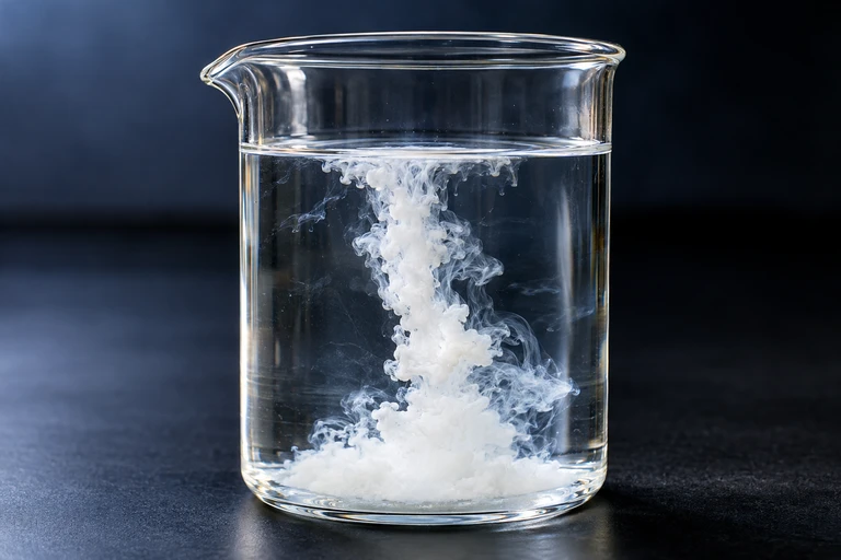
Silver chloride precipitation context Silver chloride forms a white precipitate when the dissolved ion product exceeds its solubility product.

SECTION 6

Worked Example

Let us solve a classic AP Chemistry problem: calculate the molar solubility of CaF₂ in a 0.10 M NaF solution. The K_sp of CaF₂ is 3.9 × 10⁻¹¹.

Molar Solubility of CaF₂ in 0.10 M NaF

1
Step 1 — Write the Dissolution Equation and Ksp Expression

CaF₂(s) ⇌ Ca²⁺(aq) + 2 F⁻(aq). The equilibrium expression is K_sp = [Ca²⁺][F⁻]². This is a 1:2 stoichiometry salt, so we must be careful with the coefficients.

K_sp = [Ca²⁺][F⁻]² = 3.9 × 10⁻¹¹
2
Step 2 — Set Up the ICE Table with the Common Ion

Let s = molar solubility of CaF₂. NaF is a strong electrolyte that fully dissociates, contributing 0.10 M F⁻ initially. The ICE table: [Ca²⁺] goes from 0 → +s → s; [F⁻] goes from 0.10 → +2s → (0.10 + 2s). The key difference from the pure-water case is that [F⁻] starts at 0.10, not 0.

[Ca²⁺] = s, [F⁻] = 0.10 + 2s
3
Step 3 — Apply the Simplification Assumption

Since K_sp is extremely small (3.9 × 10⁻¹¹), s will be very small compared to 0.10 M, meaning 2s ≪ 0.10. We can approximate [F⁻] ≈ 0.10 M. This eliminates the need for a cubic equation.

[F⁻] ≈ 0.10 M
4
Step 4 — Solve for s

Substituting into the K_sp expression: 3.9 × 10⁻¹¹ = s × (0.10)² = s × 0.010. Therefore s = (3.9 × 10⁻¹¹) / (0.010) = 3.9 × 10⁻⁹ M.

s = 3.9 × 10⁻⁹ M
5
Step 5 — Compare to Solubility in Pure Water

In pure water: K_sp = s(2s)² = 4s³ → s = $(3.9 × 10⁻¹¹ / 4)^{1/3}$ = $(9.75 × 10⁻¹²)^{1/3}$ ≈ 2.1 × 10⁻⁴ M. The solubility in 0.10 M NaF (3.9 × 10⁻⁹ M) is roughly 54,000 times smaller, vividly demonstrating the power of the common-ion effect.

Solubility reduced by a factor of ≈ 5.4 × 10⁴
6
Step 6 — Validate the Assumption

Check: 2s = 2 × (3.9 × 10⁻⁹) = 7.8 × 10⁻⁹ M. Compared to 0.10 M, this is negligible (7.8 × 10⁻⁸ %). The simplification was fully justified.

2s / 0.10 = 7.8 × 10⁻⁸ ≪ 5% ✓

SECTION 7

Strengths, Limitations & Common Pitfalls

While the common-ion effect provides a powerful and reliable qualitative prediction—that adding a shared ion will decrease solubility or suppress ionization—its quantitative treatment at the AP level relies on several idealizing assumptions. Understanding where these assumptions hold and where they break down is critical for earning full credit on FRQs and for developing genuine chemical intuition.

Strength	Limitation
Direct application of Le Châtelier's principle—intuitive and qualitatively reliable	Assumes ideal behavior (activity coefficients = 1); at high ionic strengths, the actual solubility may increase (salt effect or diverse-ion effect)
Simple algebraic treatment when common-ion concentration ≫ contribution from dissolution	Simplification assumption (x ≪ C₀) can fail when K is relatively large or C₀ is small; must verify the 5% rule
Predicts buffer behavior accurately via Henderson–Hasselbalch	Henderson–Hasselbalch equation breaks down when [HA] or [A⁻] is extremely dilute or when the acid is not truly weak
Useful for selective precipitation calculations (separating ions in qualitative analysis)	Does not account for complex-ion formation, which can actually increase solubility in excess reagent (e.g., AgCl in excess NH₃)

Strengths and limitations of the common-ion effect model

⚠️

WATCH OUT

The common-ion effect always decreases solubility or ionization, but two competing phenomena can work in the opposite direction. The diverse-ion (salt) effect increases solubility at high ionic strengths because inter-ionic attractions lower effective ion concentrations (activities). Meanwhile, complex-ion formation can dramatically increase solubility if the added ion forms a stable coordination complex with the metal cation. On the AP exam, look for clues like 'excess ammonia' or 'concentrated HCl' that signal complex-ion chemistry rather than a simple common-ion problem.

SECTION 8

Connection to Advanced Theory: Activity & Ionic Strength

At the AP level, we treat equilibrium expressions using molar concentrations and assume that concentration and thermodynamic activity are interchangeable. In more advanced courses—general chemistry at the honors level, analytical chemistry, and physical chemistry—this assumption is relaxed. The true equilibrium constant is expressed in terms of activities, where the activity of an ion equals the product of its molar concentration and an activity coefficient (γ). As ionic strength increases, γ drops below 1, meaning the effective concentration is lower than the stoichiometric concentration. This causes the common-ion effect to be somewhat weaker than predicted by the simple model and, in extreme cases, solubility can actually increase at very high ionic strength.

Feature	AP-Level Model	Advanced Model (Activities)
Equilibrium Expression	K_sp = [A⁺][B⁻]	K°_sp = (γ₊[A⁺])(γ₋[B⁻])
Activity Coefficients	Assumed to equal 1 (ideal dilute solution)	Calculated via Debye–Hückel equation; < 1 at high ionic strength
Ionic Strength Effect	Not considered	Higher ionic strength → lower γ → higher apparent solubility (salt effect)
Common-Ion Prediction	Always decreases solubility	Decreases solubility, but less than predicted; at very high concentrations, the salt effect may partially offset

AP-level vs. advanced treatment of the common-ion effect

For the AP exam, you need not perform activity coefficient calculations, but you should be aware that the concentration-based model is an approximation that works well in dilute solutions. If an FRQ presents data showing that experimental solubility differs from the predicted value, consider explaining the discrepancy in terms of non-ideal behavior or complex-ion formation. This kind of critical analysis can earn explanation points on long free-response questions.

SECTION 9

Practice Problems

Question 1: CONCEPTUAL

Silver chromate (Ag₂CrO₄) is a sparingly soluble salt. If AgNO₃ is added to a saturated solution of Ag₂CrO₄, which of the following best describes the immediate result?

A. The molar solubility of Ag₂CrO₄ increases because more Ag⁺ is available to react.
B. The Ksp of Ag₂CrO₄ increases to accommodate the additional Ag⁺.
C. Additional Ag₂CrO₄ precipitates as the equilibrium shifts to the left to reduce Q back to Ksp.
D. The concentration of CrO₄²⁻ increases because Ag⁺ forces more dissolution of the solid.

Show answer (C)

Correct answer: C. Adding AgNO₃ increases [Ag⁺], making the ion product Q = [Ag⁺]²[CrO₄²⁻] exceed K_sp. By Le Châtelier's principle, the equilibrium shifts toward the solid (left), causing precipitation until Q = K_sp again. Choice A is wrong because the common ion suppresses, not enhances, dissolution. Choice B is wrong because K_sp is a thermodynamic constant at a fixed temperature and does not change when concentrations change. Choice D is wrong because the shift to the left decreases [CrO₄²⁻], not increases it.

Question 2: BASIC CALCULATION

The K_sp of BaSO₄ is 1.1 × 10⁻¹⁰. What is the molar solubility of BaSO₄ in a 0.050 M Na₂SO₄ solution?

A. 1.0 × 10⁻⁵ M
B. 2.2 × 10⁻⁹ M
C. 5.5 × 10⁻¹² M
D. 1.1 × 10⁻¹⁰ M

Show answer (B)

Correct answer: B. BaSO₄ dissolves as BaSO₄(s) ⇌ Ba²⁺(aq) + SO₄²⁻(aq), so K_sp = [Ba²⁺][SO₄²⁻]. With the common ion SO₄²⁻ at 0.050 M, let s = [Ba²⁺]. Then 1.1 × 10⁻¹⁰ = s × (0.050 + s) ≈ s × 0.050, giving s = 2.2 × 10⁻⁹ M. Choice A (1.0 × 10⁻⁵) is the solubility in pure water (√K_sp), ignoring the common ion. Choice C incorrectly divides K_sp by (0.050)² rather than by 0.050. Choice D simply restates K_sp without performing any calculation.

Question 3: INTERMEDIATE

A buffer is prepared by mixing 0.30 M acetic acid (CH₃COOH, K_a = 1.8 × 10⁻⁵) with 0.50 M sodium acetate (NaCH₃COO). What is the pH of this buffer?

A. 4.52
B. 4.74
C. 4.96
D. 5.22

Show answer (C)

Correct answer: C. Using the Henderson–Hasselbalch equation: pH = pK_a + log([A⁻]/[HA]) = −log(1.8 × 10⁻⁵) + log(0.50/0.30) = 4.74 + log(1.667) = 4.74 + 0.22 = 4.96. Choice A (4.52) would result from inverting the ratio (log(0.30/0.50) = −0.22 added to 4.74). Choice B (4.74) is the pK_a itself, which would only be correct if [A⁻] = [HA]. Choice D (5.22) would arise from doubling the log term or using an incorrect K_a value.

Question 4: APPLIED

5 pts

Lead(II) iodide (PbI₂) has K_sp = 9.8 × 10⁻⁹ at 25 °C. (a) Write the balanced dissolution equation and the K_sp expression for PbI₂. (1 point) (b) Calculate the molar solubility of PbI₂ in pure water. (1 point) (c) Calculate the molar solubility of PbI₂ in a 0.20 M KI solution. State any simplifying assumptions and justify them. (2 points) (d) Explain, in terms of Le Châtelier's principle and the reaction quotient Q, why the solubility in part (c) is lower than in part (b). (1 point)

Show answer

Rubric (5 points total): (a) 1 point: PbI₂(s) ⇌ Pb²⁺(aq) + 2 I⁻(aq); K_sp = [Pb²⁺][I⁻]². Award 1 point for the correct balanced equation and correct K_sp expression (must include the squared term on [I⁻] and must omit the pure solid from the expression). (b) 1 point: Let s = molar solubility of PbI₂ in pure water. Then [Pb²⁺] = s and [I⁻] = 2s. K_sp = (s)(2s)² = 4s³ = 9.8 × 10⁻⁹. Solving: s³ = 2.45 × 10⁻⁹, so s =

(2.45 × 10⁻⁹)^{1/3}

= 1.35 × 10⁻³ M. Award 1 point for the correct ICE setup leading to 4s³ = K_sp and a correct numerical answer of approximately 1.3 × 10⁻³ M. (c) 2 points: KI is a strong electrolyte and fully dissociates, so [I⁻]_initial = 0.20 M (the common ion). Let s = molar solubility of PbI₂ in this solution. Then [Pb²⁺] = s and [I⁻] = 0.20 + 2s. Substituting into the K_sp expression: K_sp = s(0.20 + 2s)². Assume 2s ≪ 0.20, so K_sp ≈ s(0.20)² = 0.040 s. Then s = (9.8 × 10⁻⁹) / 0.040 = 2.5 × 10⁻⁷ M. Justification of assumption: 2s = 5.0 × 10⁻⁷ M, which is 0.00025% of 0.20 M, so the assumption is valid. Award 1 point for the correct algebraic setup that includes the 0.20 M common-ion concentration in the K_sp expression. Award 1 point for the correct numerical answer of 2.5 × 10⁻⁷ M with a justified simplifying assumption. (d) 1 point: When KI is added to a saturated PbI₂ solution, the concentration of I⁻ (a product ion) increases. This causes the reaction quotient Q = [Pb²⁺][I⁻]² to momentarily exceed K_sp (Q > K_sp). By Le Châtelier's principle, the system responds to the added I⁻ by shifting the equilibrium to the left (toward the solid reactant side), precipitating additional PbI₂. This shift reduces the equilibrium concentration of dissolved Pb²⁺, lowering Q back to K_sp. The net result is a lower molar solubility (2.5 × 10⁻⁷ M vs. 1.35 × 10⁻³ M), demonstrating the common-ion effect. Award 1 point for a correct explanation that references Q > K_sp upon addition of the common ion and the resulting leftward equilibrium shift that decreases solubility.

Question 5: CRITICAL THINKING

4 pts

A student dissolves AgCl in several solutions containing varying concentrations of NaCl and measures the molar solubility of AgCl. The data are shown below. [NaCl] (M) | Molar Solubility of AgCl (M) 0.000 | 1.3 × 10⁻⁵ 0.010 | 1.8 × 10⁻⁸ 0.050 | 3.6 × 10⁻⁹ 0.100 | 1.8 × 10⁻⁹ 1.000 | 2.9 × 10⁻⁸ K_sp of AgCl = 1.8 × 10⁻¹⁰ (a) Using the K_sp and the common-ion effect model, calculate the predicted molar solubility of AgCl in 0.010 M NaCl and in 0.100 M NaCl. (1 point) (b) Compare your calculated values from part (a) with the experimental data. Identify which data point(s) agree well with the model and which do not. (1 point) (c) The data at [NaCl] = 1.000 M show an increase in solubility compared to 0.100 M NaCl, which contradicts the common-ion effect prediction. Propose a chemical explanation for this anomaly. (1 point) (d) A second student claims that the K_sp must have increased at 1.000 M NaCl. Evaluate this claim. (1 point)

Show answer

Rubric (4 points total): (a) 1 point: AgCl(s) ⇌ Ag⁺(aq) + Cl⁻(aq); K_sp = [Ag⁺][Cl⁻] = 1.8 × 10⁻¹⁰. With [Cl⁻] ≈ C₀ (common ion), s ≈ K_sp/C₀. At 0.010 M NaCl: s = 1.8 × 10⁻¹⁰ / 0.010 = 1.8 × 10⁻⁸ M. At 0.100 M NaCl: s = 1.8 × 10⁻¹⁰ / 0.100 = 1.8 × 10⁻⁹ M. Award 1 point for both correct calculations. (b) 1 point: The predicted values (1.8 × 10⁻⁸ M at 0.010 M NaCl and 1.8 × 10⁻⁹ M at 0.100 M NaCl) match the experimental data exactly at those concentrations, confirming that the common-ion model works well at moderate ionic strengths. However, the model would predict s = 1.8 × 10⁻¹⁰ M at 1.000 M NaCl, whereas the experimental value is 2.9 × 10⁻⁸ M—a discrepancy of over two orders of magnitude. Award 1 point for correctly identifying agreement at lower concentrations and deviation at 1.000 M. (c) 1 point: At very high [Cl⁻], the formation of soluble complex ions such as AgCl₂⁻ (dichloroargentate) occurs: Ag⁺(aq) + 2 Cl⁻(aq) ⇌ AgCl₂⁻(aq). This complex-ion formation removes Ag⁺ from the simple equilibrium, driving additional dissolution and increasing the apparent solubility. Additionally, the high ionic strength lowers activity coefficients, contributing to the salt effect. Accept either or both explanations. Award 1 point for a chemically valid explanation. (d) 1 point: The claim is incorrect. K_sp is a thermodynamic equilibrium constant that depends only on temperature, not on the concentrations of other species in solution. The increased solubility is due to a new equilibrium (complex-ion formation) or non-ideal behavior (activity effects), not a change in K_sp. Award 1 point for correctly refuting the claim with proper reasoning about the nature of K_sp.

SUMMARY

Summary

The common-ion effect is a direct consequence of Le Châtelier's principle: when an ion that participates in an equilibrium is introduced from an external source, the reaction quotient Q momentarily exceeds the equilibrium constant, and the system shifts toward reactants to restore equilibrium. In solubility equilibria, this means the molar solubility decreases and more precipitate forms. In acid–base equilibria, the percent ionization decreases and the pH is governed by the Henderson–Hasselbalch equation, which is the foundation of buffer chemistry.

Quantitatively, solving common-ion problems requires setting up an ICE table that begins with the initial concentration of the common ion from the external source, not from zero. The simplification assumption (x ≪ C₀) is almost always valid in common-ion problems because the external ion concentration dwarfs the contribution from dissolution or ionization. Remember that Ksp and Ka are constants at a given temperature; only the concentrations adjust. At very high ionic strengths, be aware that complex-ion formation and activity effects can cause deviations from the idealized common-ion model.