Beer-Lambert Law - AP Chemistry

SECTION 1

Historical Context & Motivation

Long before modern spectrophotometers could be purchased from a catalog, scientists grappled with a deceptively simple question: how does the intensity of light change as it passes through a colored solution? The answer to this question would eventually transform analytical chemistry, enabling researchers to determine the concentration of a dissolved substance without isolating or weighing it. The Beer-Lambert Law is the mathematical relationship that emerged from over a century of careful experimentation, linking the absorption of light to both the concentration and the path length of an absorbing medium. Understanding its historical development reveals how empirical observation, combined with rigorous mathematical description, produces the quantitative tools that underpin modern chemistry.

1729 • Bouguer's Observation

Pierre Bouguer published the first systematic study of light attenuation, demonstrating that the fraction of light absorbed by a material is proportional to the thickness of the material traversed—an insight initially applied to the Earth's atmosphere.

1760 • Lambert's Formalization

Johann Heinrich Lambert placed Bouguer's observations on a firm mathematical footing, expressing the exponential decrease of light intensity with path length in his treatise Photometria. This established the logarithmic relationship between transmitted and incident light.

1852 • Beer's Extension

August Beer extended Lambert's work by showing that the attenuation of light is also proportional to the concentration of the absorbing species in solution—completing the combined law we use today.

1940s • Beckman Spectrophotometer

Arnold Beckman's development of the DU spectrophotometer made precise absorbance measurements routine, transforming Beer-Lambert calculations from a research novelty into a standard analytical technique used worldwide.

The central question these scientists pursued can be stated concisely: given a beam of monochromatic light passing through a solution, how can we predict the fraction of light that reaches the detector? And, critically, how can we reverse that calculation to determine the unknown concentration of an analyte from a simple absorbance measurement? The Beer-Lambert Law provides the elegant and quantitative answer.

SECTION 2

Core Principles & Definitions

The Beer-Lambert Law rests on several interconnected physical ideas. When a beam of light encounters a solution containing an absorbing species, three things may happen to each photon: it may pass through unaffected (transmission), it may be absorbed by a solute molecule (absorption), or it may be scattered. The Beer-Lambert Law specifically models the absorption process, assuming scattering is negligible. The fundamental idea is that each successive thin layer of solution removes the same fraction of the remaining light, which produces an exponential decay in intensity—transformed by the logarithm into a convenient linear relationship.

Absorbance (A)

A dimensionless quantity defined as A = −log₁₀(T), where T is the transmittance. Absorbance is directly proportional to both concentration and path length—this linearity is what makes the law so useful analytically.

Transmittance (T)

The ratio of transmitted light intensity (I) to incident light intensity (I₀), expressed as T = I / I₀. Transmittance ranges from 0 (all light absorbed) to 1 (no absorption), and is often reported as percent transmittance (%T = T × 100).

Molar Absorptivity (ε)

Also called the molar extinction coefficient, ε is an intrinsic property of the absorbing species at a given wavelength, with units of L·mol⁻¹·cm⁻¹. A large ε means the substance absorbs strongly at that wavelength.

Path Length (b)

The distance light travels through the solution, typically measured in centimeters. Standard cuvettes have a path length of 1.00 cm, which simplifies calculations by eliminating b from the product εbc.

Monochromatic Light

Beer-Lambert Law requires that the incident light be of a single wavelength (or a narrow band). Because ε varies with wavelength, polychromatic light produces curvature in the A vs. c plot, violating the expected linearity.

✦

KEY TAKEAWAY

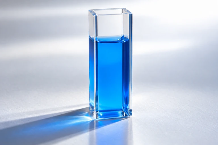Think of absorbance like walking through a fog: each meter of fog blocks the same fraction of the remaining light. A thicker fog (higher concentration) or a longer walk (longer path length) both reduce the light reaching your eyes. The Beer-Lambert Law captures this compounding attenuation as a simple linear equation: A = εbc. Because absorbance is on a logarithmic scale, the exponential loss of intensity becomes a straight line when plotted against concentration—just as a pH scale linearizes hydrogen-ion concentration.

Blue solution in an optical cuvette A blue solution transmits some visible wavelengths more strongly than others; its absorption depends on wavelength.

SECTION 3

Visual Explanation

Light Passing Through a Cuvette

The diagram shows monochromatic light of intensity I₀ entering a cuvette containing an absorbing solution of concentration c. As light traverses the path length b, absorbing molecules remove photons from the beam. The transmitted intensity I, measured at the detector, is always less than I₀. The ratio I/I₀ defines transmittance, and the negative logarithm of transmittance yields absorbance A.

In the diagram above, notice how the beam visually narrows as it passes through the sample—this represents the decrease in light intensity. Each violet circle represents an absorbing molecule; increasing the number of these molecules (raising concentration c) or increasing the distance the light must travel through them (raising path length b) both increase the total amount of light absorbed. The key insight is that absorbance A, not the raw intensity ratio, is the quantity that scales linearly with concentration—which is precisely why chemists measure absorbance rather than transmittance when constructing calibration curves.

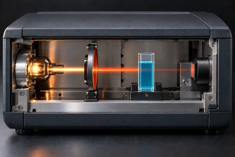One filter-based absorption photometer A photometer directs selected light through a cuvette and measures the transmitted light at a detector.

SECTION 4

Mathematical Framework

The Beer-Lambert Law is derived from the observation that each infinitesimally thin layer of solution absorbs the same fraction of light that enters it. If the intensity at depth x is I(x), then the decrease dI over an additional thickness dx is proportional to I(x) itself, to the concentration c of absorbing species, and to a proportionality constant α: dI = −α·c·I·dx. Integrating from x = 0 to x = b yields an exponential decay, which is conventionally expressed as a base-10 logarithm to give the familiar linear form.

TRANSMITTANCE

T = I / I₀

where I = transmitted light intensity and I₀ = incident light intensity. T is dimensionless, ranging from 0 to 1.

ABSORBANCE DEFINITION

A = −log₁₀(T) = −log₁₀(I / I₀)

Absorbance A is dimensionless. When T = 1 (no absorption), A = 0. When T = 0.1 (90% absorbed), A = 1. When T = 0.01 (99% absorbed), A = 2.

BEER-LAMBERT LAW

A = ε × b × c

ε = molar absorptivity (L·mol⁻¹·cm⁻¹), b = path length (cm), c = molar concentration (mol·L⁻¹). This is the central equation: absorbance is directly proportional to both concentration and path length.

SOLVING FOR CONCENTRATION

c = A / (ε × b)

This rearrangement is the most common form used in analytical chemistry. By measuring A and knowing ε (from literature or a calibration curve) and b (from the cuvette), the unknown concentration can be calculated directly.

💡

Unit Analysis

Verify dimensional consistency: ε has units L·mol⁻¹·cm⁻¹, b has units cm, and c has units mol·L⁻¹. The product εbc yields (L·mol⁻¹·cm⁻¹)(cm)(mol·L⁻¹) = dimensionless, matching the requirement that absorbance A carries no units. Always check that your units cancel properly—this is a frequent source of errors on the AP exam.

SECTION 5

Calibration Curves & Data Analysis

In practice, chemists rarely rely on a single absorbance reading and a literature value of ε to determine an unknown concentration. Instead, they construct a calibration curve (also called a standard curve or Beer's Law plot) by measuring the absorbance of several solutions of known concentration—called standard solutions. When absorbance is plotted on the y-axis against concentration on the x-axis, the Beer-Lambert Law predicts a straight line passing through the origin with slope equal to εb. A best-fit line (linear regression) through the data points allows one to read off the concentration of any unknown sample from its measured absorbance, or to extract ε from the slope when b = 1.00 cm.

A calibration curve plotting absorbance (A) against concentration for four standard solutions (amber dots). The dashed pink best-fit line passes through the origin with slope = εb. To find the concentration of an unknown (cyan dot), measure its absorbance, trace horizontally to the line, and read the concentration below.

The calibration curve above illustrates the standard analytical workflow. Four solutions of known concentration were prepared, their absorbances measured at the wavelength of maximum absorption (λ_max), and the points plotted. The best-fit line has slope εb, and its linearity confirms Beer-Lambert behavior within this concentration range. The unknown sample's absorbance is measured, then interpolated from the calibration curve to yield its concentration. Measuring at λ_max maximizes sensitivity because ε is greatest at this wavelength, producing the steepest possible calibration slope and thus the smallest uncertainty in the determined concentration.

💡

AP Exam Tip

On the AP Chemistry exam, you may be asked to determine an unknown concentration from a calibration curve or to calculate ε from the slope. Remember: if b = 1.00 cm (standard cuvette), then slope = ε numerically. Always report ε with correct units (L·mol⁻¹·cm⁻¹) and show your dimensional analysis clearly in FRQ responses.

SECTION 6

Worked Example

The following worked example demonstrates a typical Beer-Lambert calculation you might encounter on the AP Chemistry exam or in a college analytical chemistry laboratory.

Determining the Concentration of KMnO₄

1
Step 1 — Identify Given Values

A potassium permanganate (KMnO₄) solution is measured at 525 nm using a standard 1.00 cm cuvette. The spectrophotometer reads an absorbance of A = 0.740. The molar absorptivity of KMnO₄ at 525 nm is ε = 2,455 L·mol⁻¹·cm⁻¹. We need to find the molar concentration c.

A = 0.740, ε = 2,455 L·mol⁻¹·cm⁻¹, b = 1.00 cm
2
Step 2 — Write the Beer-Lambert Equation

The Beer-Lambert Law states A = εbc. We rearrange to solve for concentration: c = A / (ε × b).
3
Step 3 — Substitute Values

Substituting the known values: c = 0.740 / (2,455 L·mol⁻¹·cm⁻¹ × 1.00 cm).
4
Step 4 — Calculate and Verify Units

c = 0.740 / 2,455 = 3.015 × 10⁻⁴ mol·L⁻¹. The units work out: dimensionless / (L·mol⁻¹·cm⁻¹ × cm) = mol·L⁻¹ = M. Rounding to three significant figures (matching the precision of A), c ≈ 3.02 × 10⁻⁴ M.

c ≈ 3.02 × 10⁻⁴ mol·L⁻¹
5
Step 5 — Reasonableness Check

An absorbance of 0.740 corresponds to a transmittance of T = 10⁻⁰·⁷⁴⁰ ≈ 0.182, meaning about 18% of the incident light is transmitted. This is a moderately absorbing solution, consistent with a dilute (sub-millimolar) KMnO₄ concentration, which appears light purple—reasonable for ≈ 3 × 10⁻⁴ M.

SECTION 7

Assumptions, Strengths & Limitations

The Beer-Lambert Law is remarkably powerful, but it rests on several assumptions that, when violated, lead to deviations from linearity. Understanding these limitations is essential not only for the AP exam but also for designing reliable experiments in the laboratory. Deviations are classified as fundamental (inherent to the law itself), chemical (arising from the chemistry of the analyte), or instrumental (caused by the spectrophotometer itself).

Category	Assumption of Beer-Lambert Law	What Causes Deviation
Fundamental	Dilute solutions (absorber–absorber interactions are negligible)	At high concentrations (> ~0.01 M), solute molecules interact, changing the effective ε. The A vs. c plot curves downward.
Chemical	The analyte exists in a single absorbing form	pH-dependent equilibria, dimerization, or complexation alter the distribution of absorbing species, changing the apparent ε.
Instrumental	Monochromatic light source	A wide spectral bandwidth means ε varies across the light reaching the sample; this produces negative deviations, especially where the absorption spectrum changes rapidly.
Instrumental	No scattering or reflection losses	Turbid or colloidal solutions scatter light, inflating apparent absorbance. Dirty cuvette surfaces cause stray reflection.
Instrumental	Stray light is negligible	Stray light (light reaching the detector without passing through the sample) sets an upper limit on measurable absorbance, typically A ≈ 2–3.

Common sources of deviation from Beer-Lambert linearity

⚠️

PRACTICAL GUIDELINE

For the most reliable results, keep measured absorbance values between approximately 0.1 and 1.0. Below 0.1, the signal-to-noise ratio is poor and small errors in I dominate; above 1.0, so little light reaches the detector that stray light and detector limitations introduce significant positive bias. If your sample reads above 1.0, dilute it and measure again. This working range is a frequently tested concept on AP Chemistry free-response questions.

SECTION 8

Connections to Advanced Spectroscopy

The Beer-Lambert Law, as introduced in AP Chemistry, applies specifically to UV-visible absorption spectroscopy of solutions. However, the same underlying principle—that absorbance is proportional to the number of absorbing species in the optical path—extends across a wide range of spectroscopic and analytical techniques encountered in advanced coursework and research. Recognizing these connections helps situate the Beer-Lambert Law as a foundational quantitative tool rather than an isolated formula.

Feature	AP Chemistry (Beer-Lambert)	Advanced Techniques
Wavelength range	UV-visible (190–800 nm)	IR spectroscopy uses the same law for infrared wavelengths; X-ray absorption spectroscopy applies similar principles at much shorter wavelengths.
Sample phase	Solution (liquid)	Gas-phase spectroscopy uses the same form, substituting partial pressure or number density for molarity. Atmospheric remote sensing relies on this approach.
Multi-component	Single absorbing species	Additivity of absorbances: A_total = ε₁bc₁ + ε₂bc₂ + ··· allows simultaneous determination of multiple analytes at different wavelengths via matrix algebra.
Quantitative output	Single concentration value	Reaction kinetics: absorbance measured over time gives concentration vs. time data, enabling rate law determination—a direct connection to AP Chemistry Unit 5.

Beer-Lambert Law in AP Chemistry vs. advanced spectroscopic applications

One particularly important connection for AP Chemistry students is the use of spectrophotometry to monitor reaction rates. Because absorbance is proportional to concentration, measuring A at regular time intervals provides a real-time concentration profile without needing to withdraw and analyze samples. This technique is central to laboratory experiments on reaction kinetics and appears frequently on AP exam free-response questions that integrate spectroscopy with rate law analysis.

SECTION 9

Practice Problems

Question 1: CONCEPTUAL

A student prepares two solutions of the same dye. Solution X has twice the concentration of Solution Y. Both are measured in identical 1.00 cm cuvettes at the same wavelength. Which of the following correctly describes the relationship between their absorbance values?

A. The absorbance of X is four times the absorbance of Y because absorbance depends on the square of the concentration.
B. The absorbance of X is twice the absorbance of Y because absorbance is directly proportional to concentration.
C. The absorbance of X is half the absorbance of Y because a more concentrated solution transmits more light.
D. The absorbances of X and Y are equal because ε and b are the same for both solutions.

Show answer (B)

Correct answer: B. According to A = εbc, absorbance is directly (linearly) proportional to concentration when ε and b are constant. Doubling c doubles A. Choice A is wrong because the relationship is linear, not quadratic. Choice C reverses the relationship—higher concentration means more absorption, not less. Choice D ignores the concentration variable entirely; while ε and b are the same, c differs between the two solutions, so A must differ as well.

Question 2: BASIC CALCULATION

A solution of Co(NO₃)₂ has a molar absorptivity of 5.10 L·mol⁻¹·cm⁻¹ at 510 nm. When placed in a 1.00 cm cuvette, the solution has an absorbance of 0.357. What is the molar concentration of Co(NO₃)₂?

A. 0.0143 M
B. 0.0700 M
C. 1.82 M
D. 0.700 M

Show answer (B)

Correct answer: B. Using c = A / (εb) = 0.357 / (5.10 L·mol⁻¹·cm⁻¹ × 1.00 cm) = 0.0700 mol·L⁻¹. Choice A (0.0143 M) results from dividing A by (εb)² or making a reciprocal error. Choice C (1.82 M) would result from multiplying A × ε × b rather than dividing. Choice D (0.700 M) is off by a factor of 10, likely from a decimal placement error in ε.

Question 3: INTERMEDIATE

A calibration curve for a colored complex is constructed using a 2.00 cm cuvette. The best-fit line has the equation A = 1,240c, where c is in mol·L⁻¹. What is the molar absorptivity (ε) of the complex at the measurement wavelength?

A. 620 L·mol⁻¹·cm⁻¹
B. 1,240 L·mol⁻¹·cm⁻¹
C. 2,480 L·mol⁻¹·cm⁻¹
D. 310 L·mol⁻¹·cm⁻¹

Show answer (A)

Correct answer: A. The slope of a Beer-Lambert calibration curve (A vs. c) equals εb. Here, slope = 1,240 and b = 2.00 cm, so ε = 1,240 / 2.00 = 620 L·mol⁻¹·cm⁻¹. Choice B (1,240) incorrectly assumes b = 1.00 cm or equates the slope directly with ε. Choice C (2,480) multiplies the slope by b instead of dividing. Choice D (310) divides by b² rather than b. Students must remember that the slope equals ε only when b = 1.00 cm; otherwise, division by b is required.

Question 4: APPLIED

4 pts

A student is investigating the kinetics of the reaction between crystal violet dye and sodium hydroxide. As the reaction proceeds, the crystal violet is consumed and the solution decolorizes. The student uses a spectrophotometer set at 590 nm to monitor the reaction. (a) Explain how the absorbance measurements can be used to determine the concentration of crystal violet at each time point. (1 point) (b) The student measures the following data: Time (s): 0, 30, 60, 90, 120 Absorbance: 0.800, 0.400, 0.200, 0.100, 0.050 Using this data, determine whether the reaction is first order with respect to crystal violet. Justify your answer quantitatively. (2 points) (c) If NaOH is present in large excess, explain why the experiment effectively monitors only the order with respect to crystal violet. (1 point)

Show answer

Rubric (4 points): Part (a) — 1 point: According to Beer-Lambert Law (A = εbc), absorbance is directly proportional to the concentration of crystal violet. With ε and b constant throughout the experiment, concentration at any time is proportional to A: c = A / (εb). Alternatively, a calibration curve of known crystal violet concentrations vs. absorbance could be used to convert each A reading to a concentration. (1 pt for stating the proportional relationship or citing A = εbc and correctly linking A to c.) Part (b) — 2 points: For a first-order reaction, the half-life is constant. Examining the data: A drops from 0.800 to 0.400 in 30 s (first half-life), from 0.400 to 0.200 in 30 s (second half-life), from 0.200 to 0.100 in 30 s (third half-life), and from 0.100 to 0.050 in 30 s (fourth half-life). The constant half-life of 30 s confirms first-order behavior. Alternatively, ln(A) vs. t should be linear for a first-order process: ln(0.800) = −0.223, ln(0.400) = −0.916, ln(0.200) = −1.609, ln(0.100) = −2.303, ln(0.050) = −2.996. The differences in ln(A) per 30 s interval are each approximately −0.693, confirming linearity. (1 pt for correct quantitative analysis showing constant half-life or linear ln(A) vs. t; 1 pt for explicitly stating the conclusion that the reaction is first order with respect to crystal violet.) Part (c) — 1 point: When NaOH is present in large excess, its concentration remains essentially constant throughout the reaction (pseudo-order conditions). The rate law simplifies from rate = k[CV⁺][OH⁻]ⁿ to rate = k'[CV⁺], where k' = k[OH⁻]ⁿ is a pseudo-rate constant. Therefore, changes in absorbance over time reflect only the changing crystal violet concentration, allowing determination of its reaction order in isolation. (1 pt for explaining pseudo-order conditions and how constant [OH⁻] isolates the crystal violet dependence.)

Question 5: CRITICAL THINKING

4 pts

A student prepares six standard solutions of an iron(III)–thiocyanate complex and measures their absorbance at 447 nm using a 1.00 cm cuvette. The data are shown below: | Concentration (× 10⁻⁴ M) | Absorbance | |---|---| | 0.50 | 0.110 | | 1.00 | 0.215 | | 2.00 | 0.430 | | 3.00 | 0.648 | | 5.00 | 0.975 | | 8.00 | 1.320 | (a) Plot these data mentally (or on scratch paper) and describe the shape of the graph. Does Beer's Law hold over the entire concentration range? Justify your answer. (2 points) (b) Using only the data points that obey Beer's Law, estimate the molar absorptivity ε of the complex at 447 nm. Show your calculation. (1 point) (c) An unknown solution measured under the same conditions gives A = 0.540. Determine the concentration of the iron(III)–thiocyanate complex. Is it appropriate to use your Beer's Law calibration for this measurement? Explain. (1 point)

Show answer

Rubric (4 points): Part (a) — 2 points: (1 pt) For the first four points (0.50 to 3.00 × 10⁻⁴ M), the ratio A/c is approximately constant: 0.110/0.50 = 0.220 × 10⁴, 0.215/1.00 = 0.215 × 10⁴, 0.430/2.00 = 0.215 × 10⁴, 0.648/3.00 = 0.216 × 10⁴. These are linear and consistent with Beer's Law. (1 pt) However, at 5.00 × 10⁻⁴ M, the ratio drops: 0.975/5.00 = 0.195 × 10⁴, and at 8.00 × 10⁻⁴ M: 1.320/8.00 = 0.165 × 10⁴. The curve shows negative deviation (bending downward) at higher concentrations, indicating Beer's Law breaks down—likely due to molecular interactions at higher concentration or the absorbance approaching the reliable measurement limit. Part (b) — 1 point: Using the linear region (first four data points), the slope = A/c ≈ 0.216 × 10⁴ = 2,160. Since b = 1.00 cm, slope = εb = ε. Therefore ε ≈ 2,160 L·mol⁻¹·cm⁻¹. (Alternatively, one may calculate the slope from any two points in the linear range, e.g., (0.430 − 0.110)/(2.00 − 0.50) × 10⁴ = 0.320/1.50 × 10⁴ = 2,133 ≈ 2,100 L·mol⁻¹·cm⁻¹. Accept values in the range 2,100–2,200.) (1 pt for a correct calculation with appropriate data selection.) Part (c) — 1 point: Using c = A / (εb) = 0.540 / (2,160 × 1.00) = 2.50 × 10⁻⁴ M. This absorbance value (0.540) falls within the linear range (between 0.430 at 2.00 × 10⁻⁴ M and 0.648 at 3.00 × 10⁻⁴ M), so interpolation from the Beer's Law calibration is appropriate. Had the absorbance been above ~0.65 (the boundary of the linear region), the student should not have used the linear calibration—they would need to dilute the sample first. (1 pt for correct concentration calculation AND justification that the value falls within the linear range.)

SUMMARY

Beer-Lambert Law — Summary

Summary

The Beer-Lambert Law establishes that absorbance (A) is directly proportional to the product of molar absorptivity (ε), path length (b), and concentration (c), expressed as A = εbc. Transmittance (T = I/I₀) is the fraction of light passing through the sample, and absorbance is its negative base-10 logarithm. Because absorbance scales linearly with concentration, a calibration curve (A vs. c) allows determination of unknown concentrations by interpolation.

The law holds under specific conditions: dilute solutions, monochromatic light, no scattering, and a single absorbing species. Deviations arise at high concentrations, with polychromatic sources, or when chemical equilibria shift the identity of the absorber. For reliable measurements, keep absorbance between 0.1 and 1.0. On the AP Chemistry exam, expect questions that require calculating concentration from absorbance data, interpreting calibration curves, extracting molar absorptivity from slope data, and connecting spectrophotometry to reaction kinetics.