01 / 20

Logistic Models with
Differential Equations

Master the S-shaped curve that models bounded growth: from the differential equation \(\frac{dP}{dt}=kP\!\left(1-\frac{P}{L}\right)\) to its closed-form solution and AP-style applications.

AP Calculus BC

What Is Logistic Growth?

In nature, populations don't grow forever. Resources are finite: food, space, and energy impose limits. Logistic growth describes a population that grows quickly at first, then slows down as it approaches an upper bound called the carrying capacity.

The S-Curve Visualized

Phase 1
Near-exponential growth when \(P \ll L\)
Phase 2
Inflection at \(P = \frac{L}{2}\): fastest growth rate
Phase 3
Growth decelerates; \(P \to L\) as \(t \to \infty\)

Key Terms to Know

1
Carrying Capacity \(L\): The maximum population the environment can sustain. As \(P \to L\), growth rate \(\to 0\).
2
Growth Constant \(k\): Controls how fast the population grows. Larger \(k\) means a steeper S-curve.
3
Inflection Point: Occurs at \(P = \frac{L}{2}\). This is where \(\frac{d^2P}{dt^2} = 0\) and the population grows fastest.
4
Equilibrium Solutions: \(P = 0\) (unstable) and \(P = L\) (stable). The population settles at \(L\).

The Core Differential Equation

The Closed-Form Solution

Separating variables and integrating with partial fractions yields the explicit solution:

Key properties of this solution:

\(t = 0\)
\(P(0) = \frac{L}{1+A} = P_0\) ✓
\(t \to \infty\)
\(e^{-kt} \to 0\), so \(P \to L\)

Exponential vs Logistic

Exponential Logistic
DE \(\frac{dP}{dt} = kP\) \(\frac{dP}{dt} = kP\!\left(1 - \frac{P}{L}\right)\)
Solution \(P = P_0 e^{kt}\) \(P = \frac{L}{1 + Ae^{-kt}}\)
Long-term \(P \to \infty\) \(P \to L\)
Shape J-curve (unbounded) S-curve (bounded)
Inflection None At \(P = L/2\)

Finding the Inflection Point

The inflection point is where the rate of growth is maximized: where \(\frac{d^2P}{dt^2} = 0\).

1
Start with: \(\frac{dP}{dt} = kP - \frac{k}{L}P^2\)
2
Differentiate again: \(\frac{d^2P}{dt^2} = k\frac{dP}{dt} - \frac{2k}{L}P\frac{dP}{dt} = \frac{dP}{dt}\!\left(k - \frac{2kP}{L}\right)\)
3
Set equal to zero: Since \(\frac{dP}{dt} \neq 0\) at inflection, we need \(k - \frac{2kP}{L} = 0\), giving \(P = \frac{L}{2}\).

An aquarium window connects population to growth rate

Caretaker, aerator, habitat shelf, vegetation and fish establish a managed pond. Visible fish are illustrative individuals, not the model initial population or carrying capacity. Separate exact panel: Separate computed plots show a population trajectory from1000 toward8000 and a growth-rate parabola peaking at4000 with1000fish per year.For P′ = 0.5P(1 − P/8,000) with P(0) = 1,000, the population approaches 8,000 fish. Growth is fastest at 4,000 fish, about 3.89 years after the start.

For the stated increasing logistic trajectory growth rate peaks atP=4000 fish.
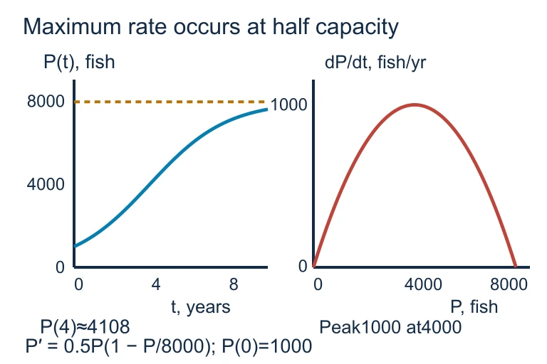
For P′ = 0.5P(1 − P/8,000) with P(0) = 1,000, the population approaches 8,000 fish. Growth is fastest at 4,000 fish, about 3.89 years after the start.For P′ = 0.5P(1 − P/8,000) with P(0) = 1,000, the population approaches 8,000 fish. Growth is fastest at 4,000 fish, about 3.89 years after the start.

How to Apply the Logistic Model

1
Identify the DE form: Confirm it matches \(\frac{dP}{dt} = kP\!\left(1 - \frac{P}{L}\right)\). Read off \(k\) and \(L\).
2
Find \(A\): Use the initial condition \(P(0) = P_0\) to compute \(A = \frac{L - P_0}{P_0}\).
3
Write the solution: \(P(t) = \frac{L}{1 + Ae^{-kt}}\).
4
Answer the question: Find \(P\) at a specific \(t\), the time to reach a given \(P\), the max growth rate at \(P = L/2\), or \(\lim_{t\to\infty} P(t) = L\).

Example 1: Reading the DE

1
Identify: \(k = \) 0.4, \(L = \) 5000.
2
Compute \(A\): \(A = \frac{5000 - 500}{500} = \frac{4500}{500} = \) 9.
3
Solution: \(P(t) = \frac{5000}{1 + 9e^{-0.4t}}\).
4
Long-term: \(\lim_{t\to\infty} P(t) = \) 5000.

Example 2: Max Growth Rate

1
Max growth at inflection: \(P = \frac{L}{2} = \frac{5000}{2} = \) 2500.
2
Substitute: \(\frac{dP}{dt}\bigg|_{P=2500} = 0.4(2500)\!\left(1 - \frac{2500}{5000}\right)\).
3
Simplify: \(= 0.4 \times 2500 \times 0.5 = \) 500 fish/unit time.

Example 3: Factored Form

1
Factor: \(\frac{dP}{dt} = 3P - 0.01P^2 = P(3 - 0.01P) = 3P\!\left(1 - \frac{P}{300}\right)\).
2
Read off: \(k = \) 3, \(L = \) 300.
3
Max growth at: \(P = \frac{300}{2} = \) 150.
4
Max rate: \(\frac{kL}{4} = \frac{3 \times 300}{4} = \) 225 per unit time.

Slope Fields and Logistic Curves

A population above carrying capacity decreases
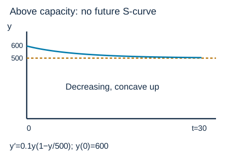
A population curve starts at 600 above the dashed carrying-capacity line 500 and decreases toward it from above, flattening as time advances.For y′ = 0.1 y(1 − y/500) with y(0) = 600, the initial rate is −12. The solution decreases toward 500 and is concave up for all future time; this trajectory has no future inflection point.Open full diagram

Separating the Logistic DE

The AP exam may ask you to set up (not always fully solve) the separation of variables:

1
Separate: \(\dfrac{dP}{P\!\left(1 - \frac{P}{L}\right)} = k\,dt\)
2
Partial fractions: \(\dfrac{1}{P\!\left(1 - \frac{P}{L}\right)} = \dfrac{1}{P} + \dfrac{1/L}{1 - P/L}\)
3
Integrate both sides: \(\ln|P| - \ln\!\left|1 - \frac{P}{L}\right| = kt + C\)
4
Solve for \(P\): Exponentiate and apply initial condition to get \(P(t) = \frac{L}{1 + Ae^{-kt}}\).

Common Mistakes to Avoid

✕ Misreading \(k\) vs \(k/L\)
Given \(\frac{dP}{dt} = 3P - 0.01P^2\), students say \(k = 0.01\). You must factor to standard form first: \(k = 3\), \(L = 300\).
✕ Wrong Inflection Point
Inflection is at \(P = L/2\), not \(t = L/2\). It is a population value, not a time value.
✕ Forgetting the Limit
\(\lim_{t\to\infty} P(t) = L\), not \(\infty\). The logistic model is bounded. Never write \(P \to \infty\).

Summary Cheat Sheet

Property Value / Formula
DE \(\frac{dP}{dt} = kP\!\left(1 - \frac{P}{L}\right)\)
Solution \(P(t) = \frac{L}{1 + Ae^{-kt}}\)
Constant \(A\) \(A = \frac{L - P_0}{P_0}\)
Carrying Capacity \(\lim_{t\to\infty} P(t) = L\)
Inflection Point \(P = \frac{L}{2}\)
Max Growth Rate \(\frac{kL}{4}\)
Equilibria \(P = 0\) (unstable), \(P = L\) (stable)

Question 1 of 5

A population satisfies \(\dfrac{dP}{dt} = 0.5P\!\left(1 - \dfrac{P}{800}\right)\). What is the carrying capacity?

Question 2 of 5

For the logistic equation \(\dfrac{dP}{dt} = 2P - 0.004P^2\), what are \(k\) and \(L\)?

Question 3 of 5

A logistic model has \(k = 0.6\) and \(L = 1000\). At what population is the rate of growth greatest?

Question 4 of 5

If \(P(0) = 100\) and \(L = 2000\), what is the value of \(A\) in the solution \(P(t) = \dfrac{L}{1 + Ae^{-kt}}\)?

Question 5 of 5

Given \(\dfrac{dP}{dt} = 0.3P\!\left(1 - \dfrac{P}{600}\right)\), what is the maximum possible value of \(\dfrac{dP}{dt}\)?