Solving Optimization Problems - AP Calculus BC

SECTION 1

Historical Context & Motivation

The desire to find the "best" outcome—the largest area, the shortest path, the least cost—has driven mathematical inquiry for millennia. Ancient Greek mathematicians wrestled with problems like enclosing the maximum area with a fixed perimeter, a question known as the isoperimetric problem. However, without a systematic tool for locating extrema, solutions relied on geometric insight and ad hoc argument. The invention of calculus in the seventeenth century transformed optimization from a collection of clever tricks into a general, algorithmic discipline. By connecting the sign of a derivative to the increase or decrease of a function, Newton and Leibniz gave mathematicians—and later engineers, economists, and scientists—a universal method for identifying maximum and minimum values.

~300 BCE • Euclid & Greek Extrema

Euclid showed that among all rectangles with a given perimeter, the square has the greatest area—one of the earliest recorded optimization results, proved purely by geometric reasoning.

1638 • Fermat's Method of Adequality

Pierre de Fermat developed a proto-derivative technique called adequality to find tangent lines and extrema, foreshadowing the first-derivative test by several decades.

1684 • Leibniz Publishes Calculus

Gottfried Wilhelm Leibniz published his differential calculus, providing the dy/dx notation and formal rules for differentiation that made optimization problems routine.

1696 • The Brachistochrone Problem

Johann Bernoulli posed the brachistochrone challenge—find the curve of fastest descent under gravity—sparking the development of the calculus of variations, an advanced generalization of optimization.

Modern Era • Industrial & Computational Optimization

Today, optimization pervades machine learning, operations research, and engineering design. The single-variable techniques you learn in AP Calculus BC remain the conceptual foundation for all of these multivariable and numerical methods.

The central question this lesson addresses is deceptively simple: given a real-world quantity that depends on one or more variables, and given constraints that restrict those variables, how do we systematically determine the absolute maximum or minimum of that quantity? The answer lies in translating the verbal description into a single-variable function, applying derivative tests, and verifying that the critical point yields a global—not merely local—extremum.

SECTION 2

Core Principles of Optimization

Every optimization problem in calculus follows a predictable logical arc. You begin by understanding the physical or geometric scenario, identify the quantity to be optimized, express it as a function of a single variable, find critical points via differentiation, and then confirm that your candidate is indeed the global extremum on the relevant domain. Mastering these steps converts even intimidating word problems into manageable algebra and calculus.

Identify the Objective Function

Determine which quantity (area, volume, cost, distance, time, etc.) you are asked to maximize or minimize. Write an expression for it in terms of available variables.

Establish the Constraint

Identify the equation or inequality that restricts the variables. Use the constraint to eliminate all but one independent variable from the objective function.

Determine the Domain

Physical context dictates admissible values. Lengths must be positive, angles may be bounded, and percentages stay between 0 and 1. Define a closed or open interval for your variable.

Differentiate and Find Critical Points

Set the first derivative equal to zero and solve. Also check where the derivative is undefined. These candidates, along with domain endpoints, are the only places where an extremum can occur.

Verify the Global Extremum

Use the Closed Interval Method (compare function values at critical points and endpoints), the First Derivative Test, or the Second Derivative Test to confirm your answer is the absolute max or min.

✦

KEY TAKEAWAY

Think of an optimization problem like tuning a radio dial: the constraint fixes which stations are available (the domain), and the derivative tells you which direction to turn to improve the signal. The critical point where the derivative equals zero is the station that comes in clearest—the optimal solution.

SECTION 3

Visual Explanation — The Optimization Workflow

The following diagram illustrates the complete optimization workflow as a flowchart. Each stage corresponds to one of the core principles from Section 2. Following these steps in order ensures that you translate the word problem faithfully, reduce the problem to single-variable calculus, and arrive at a verified global extremum.

The six-step optimization workflow. Steps 1–4 are algebraic setup; Steps 5–6 are calculus. Most errors on the AP exam occur in the setup phase, so invest time in writing clear equations before differentiating.

Notice that the flowchart separates the algebraic modeling (steps 1–4) from the calculus execution (steps 5–6). On the AP exam, the modeling phase is typically where points are lost. Students who rush to differentiate before correctly writing the objective function and eliminating variables often optimize the wrong quantity or produce an expression in two variables that cannot be differentiated with respect to a single variable. A careful, methodical approach to setup prevents these costly errors.

SECTION 4

Mathematical Framework

The theoretical backbone of optimization is the Extreme Value Theorem: if f is continuous on a closed interval [a, b], then f attains both an absolute maximum and an absolute minimum on that interval. These extreme values must occur at critical points in the interior or at the endpoints. When the domain is not a closed interval—say, an open interval or a half-line—we rely on derivative tests and limiting behavior to confirm that a critical point delivers a global extremum.

EXTREME VALUE THEOREM

If f is continuous on [a, b], then ∃ c, d ∈ [a, b] such that f(c) ≤ f(x) ≤ f(d) for all x ∈ [a, b].

Here c is the location of the absolute minimum and d is the location of the absolute maximum on the interval.

FIRST DERIVATIVE CONDITION

f ′(x) = 0 or f ′(x) does not exist ⟹ x is a critical point.

All local (and hence global) extrema of a differentiable function occur at critical points. However, not every critical point is an extremum—always verify.

SECOND DERIVATIVE TEST

If f ′(c) = 0 and f ″(c) > 0, then f has a local minimum at c. If f ″(c) < 0, then f has a local maximum at c.

If f ″(c) = 0, the test is inconclusive; use the First Derivative Test or higher-order derivatives instead.

CLOSED INTERVAL METHOD

Absolute max/min of f on [a, b] = max/min { f(a), f(c₁), f(c₂), …, f(b) }

Evaluate f at every critical point c₁, c₂, … inside (a, b) and at both endpoints a and b. Compare all values. The largest is the absolute maximum; the smallest is the absolute minimum.

💡

AP Exam Tip

On the free-response section, you must justify that your critical point yields an absolute extremum, not just a local one. State the method you are using (Closed Interval Method, Second Derivative Test, or sign-chart First Derivative Test) and show the supporting computation. Simply stating "f ′(c) = 0 so c is a max" earns no justification credit.

SECTION 5

Common Optimization Problem Types

Although optimization problems appear in endless real-world guises, the AP Calculus BC exam draws from a relatively small family of recurring problem types. Recognizing which family a problem belongs to immediately suggests the correct geometric or algebraic setup. The diagram below classifies these families, and the table that follows summarizes the typical objective function and constraint for each.

Five recurring families of optimization problems. Recognizing the family helps you set up the objective function and constraint quickly, which is especially valuable under time pressure on the AP exam.

Problem Family	Typical Objective	Typical Constraint	Key Tip
Geometric (inscribed shapes)	Maximize area or perimeter	Point lies on a given curve	Substitute y = f(x) directly into the area formula
Container / Box	Minimize surface area or material	Fixed volume	Solve the volume constraint for h and substitute into surface area
Distance / Path	Minimize distance or squared distance	Point constrained to a curve	Minimize D² instead of D to avoid the square root
Economic / Cost	Maximize profit P(x) = R(x) − C(x)	Production capacity 0 ≤ x ≤ N	P ′(x) = 0 ⟹ marginal revenue = marginal cost
Time / Rate (Snell's Law type)	Minimize total travel time	Two different speeds in two media	Express distances via Pythagorean theorem in terms of entry point

Summary of the five main optimization problem families and their setup strategies.

SECTION 6

Worked Example — Open-Top Box Problem

A manufacturer needs to construct an open-top rectangular box with a square base from 1200 cm² of sheet metal. Find the dimensions that maximize the volume of the box.

Maximize the Volume of an Open-Top Box

1
Step 1 — Identify Variables and Draw

Let the side length of the square base be x cm and the height of the box be h cm. The box has one square base (area x²) and four rectangular sides (each of area x × h). There is no top.
2
Step 2 — Write the Objective Function

The volume to maximize is V = x² × h. This currently depends on two variables, so we need the constraint to eliminate one.
3
Step 3 — Write the Constraint and Reduce to One Variable

The total surface area of the open-top box is: S = x² + 4xh = 1200. Solving for h: h = (1200 − x²) / (4x). Substituting into V: V(x) = x² × (1200 − x²) / (4x) = x(1200 − x²) / 4 = 300x − x³/4.

V(x) = 300x − x³/4
4
Step 4 — Determine the Domain

Physical constraints require x > 0 and h > 0. Since h = (1200 − x²)/(4x) > 0, we need x² < 1200, so x < √1200 = 20√3 ≈ 34.64. Also, when x = 0 or x = 20√3, the volume is zero. Thus the domain is the open interval (0, 20√3), but V → 0 at both endpoints, guaranteeing any interior maximum is the global maximum.

Domain: 0 < x < 20√3
5
Step 5 — Differentiate and Find Critical Points

V ′(x) = 300 − 3x²/4. Set V ′(x) = 0: 300 − 3x²/4 = 0 → 3x²/4 = 300 → x² = 400 → x = 20 (taking the positive root since x > 0).

Critical point: x = 20 cm
6
Step 6 — Verify Global Maximum (Second Derivative Test)

V ″(x) = −3x/2. At x = 20: V ″(20) = −3(20)/2 = −30 < 0. Since V ″(20) < 0, the function is concave down at x = 20, confirming a local maximum. Because this is the only critical point on the interval and V → 0 at both ends of the domain, this local maximum is also the absolute maximum.

V ″(20) = −30 < 0 → confirmed maximum
7
Step 7 — Compute the Optimal Dimensions and Volume

With x = 20: h = (1200 − 400)/(4 × 20) = 800/80 = 10 cm. Volume: V = 20² × 10 = 4000 cm³.

Optimal dimensions: 20 cm × 20 cm × 10 cm, giving V = 4000 cm³

⚠

Common Mistake

A frequent error is forgetting that an open-top box has surface area x² + 4xh, not 2x² + 4xh (which would be a closed box). Always re-read the problem statement to check whether surfaces are missing, sealed, or combined.

A cardboard net with four corner squares removed, partly folded walls, and a finished open-top box on a worktable. For an open-top square-base box with 1,200 cm² of material, x² + 4xh = 1,200. Volume is largest at base side 20 cm and height 10 cm, giving 4,000 cm³.

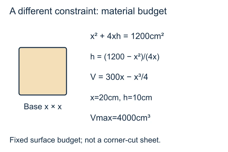For an open-top square-base box with 1,200 cm² of material, x² + 4xh = 1,200. Volume is largest at base side 20 cm and height 10 cm, giving 4,000 cm³.

SECTION 7

Comparing Verification Methods

After finding a critical point, you must verify that it gives a global extremum, not merely a local one. Three standard verification strategies are available, each with distinct strengths and limitations. Choosing the right one depends on whether the domain is a closed interval, whether the second derivative is easy to compute, and how many critical points exist.

Method	Procedure	When to Use	Limitations
Closed Interval Method	Evaluate f at all critical points and both endpoints; compare values.	Domain is a closed interval [a, b] and f is continuous.	Cannot be used on open or unbounded domains.
First Derivative Test	Analyze the sign of f ′ on intervals around the critical point.	Any domain; especially useful when f ″ is hard to compute.	Confirms local extremum; need additional argument for global.
Second Derivative Test	Compute f ″(c); sign determines concavity and thus local max or min.	f ″ is easy to compute and f ″(c) ≠ 0.	Inconclusive when f ″(c) = 0; only confirms local, not global, unless additional reasoning is provided.

Comparison of three standard verification strategies for extrema.

✦

KEY TAKEAWAY

When there is only one critical point on an interval and the function's values approach the same limit (or worse values) at the boundary, that single critical point must be the global extremum. This is the "single critical point" argument, and it is the most efficient justification on the AP exam for open-domain optimization problems—analogous to knowing that the only summit on a mountain must be the highest point.

SECTION 8

Connections to Advanced Theory

The single-variable optimization techniques in AP Calculus BC form the gateway to much deeper optimization theory. In multivariable calculus, the gradient replaces the derivative, and the method of Lagrange multipliers generalizes the constraint-elimination step you learned here. In the calculus of variations, the unknown is an entire function rather than a single number, and the Euler–Lagrange equation plays the role of setting the derivative to zero. Understanding the logical skeleton of single-variable optimization—objective, constraint, critical point, verification—prepares you for all of these extensions.

Concept	AP Calculus BC (Single Variable)	Advanced Extension
Critical point condition	f ′(x) = 0	∇f = 0 (gradient equals zero vector in ℝⁿ)
Constraint handling	Substitute constraint into objective to reduce variables	Lagrange multipliers: ∇f = λ∇g (no substitution needed)
Second-order verification	Sign of f ″(c)	Sign-definiteness of the Hessian matrix
Functional optimization	Not covered	Calculus of variations: Euler–Lagrange equation

How single-variable optimization concepts generalize in advanced mathematics.

For the AP exam, the key insight is that every optimization problem ultimately reduces to finding where a derivative (or gradient) is zero and then checking a second-order condition. If you internalize this pattern now, the multivariable generalization in college will feel like a natural broadening of familiar ideas rather than an entirely new subject.

SECTION 9

Practice Problems

Question 1: CONCEPTUAL

A continuous function f is defined on the closed interval [2, 8] and has exactly one critical point at x = 5, where f(5) = 12. If f(2) = 3 and f(8) = 7, what is the absolute maximum value of f on [2, 8]?

A. 3
B. 7
C. 12
D. It cannot be determined without knowing f ′(5).
E. It cannot be determined without knowing f on the entire interval.

Show answer (C)

By the Closed Interval Method, the absolute maximum of a continuous function on a closed interval must occur at a critical point or at an endpoint. The candidates are f(2) = 3, f(5) = 12, and f(8) = 7. Comparing these values, the absolute maximum is 12 at x = 5. This problem tests whether students understand the Extreme Value Theorem and the Closed Interval Method without requiring any differentiation.

Question 2: BASIC CALCULATION

Find two positive numbers whose sum is 50 and whose product is a maximum.

A. 10 and 40, with product 400
B. 20 and 30, with product 600
C. 25 and 25, with product 625
D. 15 and 35, with product 525
E. 1 and 49, with product 49

Show answer (C)

Let the two numbers be x and 50 − x, where 0 < x < 50. The product is P(x) = x(50 − x) = 50x − x². Taking the derivative: P ′(x) = 50 − 2x. Setting P ′(x) = 0 gives x = 25. Since P ″(x) = −2 < 0, this is a maximum. Both numbers equal 25, and the maximum product is 25 × 25 = 625. This classic result illustrates the AM-GM inequality: for a fixed sum, the product is maximized when the terms are equal.

Question 3: INTERMEDIATE

A farmer has 600 meters of fencing and wants to enclose a rectangular field bordered on one side by a river (no fence needed on the river side). What are the dimensions of the field that maximize the enclosed area?

A. 200 m × 200 m = 40,000 m²
B. 300 m × 150 m = 45,000 m²
C. 400 m × 100 m = 40,000 m²
D. 250 m × 175 m = 43,750 m²
E. 600 m × 0 m = 0 m²

Show answer (B)

Let x be the length of the side parallel to the river and y be the length of each of the two sides perpendicular to the river. The fencing constraint is x + 2y = 600, so x = 600 − 2y. The area is A = x × y = (600 − 2y)y = 600y − 2y². Taking the derivative: A ′(y) = 600 − 4y. Setting A ′(y) = 0 gives y = 150 m, and x = 600 − 2(150) = 300 m. Since A ″(y) = −4 < 0, this is a maximum. The maximum area is 300 × 150 = 45,000 m². The key strategy choice was which variable to solve for in the constraint; either works, but solving for x avoids fractions.

Question 4: APPLIED

4 pts

A cylindrical can (with a top and bottom) must hold exactly 500π cm³ of liquid. The material for the top and bottom costs $0.06 per cm² and the material for the curved side costs $0.03 per cm². Find the radius r and height h that minimize the total cost of materials. Justify that your answer gives an absolute minimum.

Show answer

(a) [1 point] Volume constraint: πr²h = 500π, so h = 500/r². (b) [1 point] Cost function: The top and bottom have combined area 2πr², costing 0.06(2πr²) = 0.12πr². The lateral surface has area 2πrh, costing 0.03(2πrh) = 0.06πrh. Total cost: C(r) = 0.12πr² + 0.06πr(500/r²) = 0.12πr² + 30π/r, for r > 0. (c) [1 point] Differentiation: C ′(r) = 0.24πr − 30π/r². Setting C ′(r) = 0: 0.24πr = 30π/r², so r³ = 30/0.24 = 125, hence r = 5 cm. Then h = 500/25 = 20 cm. (d) [1 point] Verification: C ″(r) = 0.24π + 60π/r³. At r = 5: C ″(5) = 0.24π + 60π/125 = 0.24π + 0.48π = 0.72π > 0. Since C ″(5) > 0, the function is concave up at r = 5, confirming a local minimum. Because this is the only critical point on (0, ∞) and C(r) → ∞ as r → 0⁺ and as r → ∞, this local minimum is the absolute minimum. Optimal dimensions: r = 5 cm, h = 20 cm.

Question 5: CRITICAL THINKING

3 pts

Let f(x) = x³ − 12x + 1 on the interval [−3, 5]. A student claims that the absolute minimum of f on this interval occurs at x = 2 because f ′(2) = 0 and f ″(2) = 12 > 0. Identify the error in this reasoning and determine the correct absolute minimum value.

Show answer

(a) [1 point] The student's error: The Second Derivative Test at x = 2 only confirms that x = 2 is a local minimum, not necessarily the absolute minimum on [−3, 5]. On a closed interval, the Closed Interval Method requires evaluating f at all critical points AND both endpoints. (b) [1 point] Finding all critical points: f ′(x) = 3x² − 12 = 0 gives x² = 4, so x = −2 and x = 2. Both lie in [−3, 5]. (c) [1 point] Evaluating f at critical points and endpoints: f(−3) = −27 + 36 + 1 = 10; f(−2) = −8 + 24 + 1 = 17; f(2) = 8 − 24 + 1 = −15; f(5) = 125 − 60 + 1 = 66. Comparing: the absolute minimum is f(2) = −15, and the absolute maximum is f(5) = 66. In this case, the student's answer happened to be correct, but the reasoning was flawed. On the AP exam, incomplete justification—omitting the comparison with endpoints—loses the justification point even if the numerical answer is correct.

SUMMARY

Lesson Summary

Summary

Solving optimization problems in calculus requires a systematic approach: identify the objective function (the quantity to maximize or minimize), use the constraint to reduce the problem to a single variable, determine the feasible domain, find critical points by setting the first derivative equal to zero, and verify the global extremum using the Closed Interval Method, the First Derivative Test, or the Second Derivative Test.

The Extreme Value Theorem guarantees that a continuous function on a closed interval attains its absolute maximum and minimum. On open or unbounded domains, the single critical point argument—combined with behavior at the boundary—provides the necessary justification. Common problem families include geometric, container, distance, and economic optimization, and recognizing the family accelerates setup. Always justify your answer on the AP exam—stating the method and showing the computation that confirms a global extremum is essential for earning full credit.