Representing Series as Power Series - AP Calculus BC

SECTION 1

Historical Context & Motivation

Long before modern computing, mathematicians sought ways to express complicated functions—logarithms, trigonometric ratios, and exponentials—as infinite sums of simpler polynomial terms. The idea that a function could be "unfolded" into an endless series of powers of x was both philosophically bold and practically transformative. Power series became the bridge between algebra and analysis, allowing mathematicians to compute values, prove convergence, and solve differential equations that had no closed-form solutions. Understanding this history clarifies why the AP Calculus BC curriculum treats power series representation as a capstone topic in the study of infinite sequences and series.

1668 • Mercator's Series for ln(1 + x)

Nicolaus Mercator published the series ln(1 + x) = x − x²/2 + x³/3 − ⋯, one of the earliest explicit power series representations of a transcendental function.

1715 • Brook Taylor's General Formula

Brook Taylor formalized the idea that a smooth function could be expanded around a point as a sum of derivatives weighted by powers of (x − a), laying the groundwork for all Taylor and Maclaurin series.

1742 • Colin Maclaurin's Treatise

Maclaurin systematized the special case of Taylor series centered at a = 0, producing the Maclaurin series that AP students encounter frequently—e.g., for eˣ, sin x, and cos x.

1821 • Cauchy Introduces Rigorous Convergence

Augustin-Louis Cauchy established formal convergence criteria including the ratio test, finally giving power series a rigorous analytic foundation and defining the radius of convergence.

The central question these mathematicians were answering—and the one this lesson addresses—is deceptively simple: Can we rewrite a known function as a power series, and if so, how do we find the series and determine where it converges? Mastering this skill will let you convert rational functions, logarithms, and other expressions into power series by leveraging the geometric series template and algebraic manipulation, without computing a single derivative.

SECTION 2

Core Principles & Definitions

Before diving into techniques, it is essential to establish the definitions and foundational facts that make power series representations possible. A power series centered at c is an infinite series of the form Σ aₙ(x − c)ⁿ for n = 0, 1, 2, …, where each aₙ is a constant coefficient. When c = 0, we often call the result a Maclaurin series. The entire strategy of "representing a function as a power series" rests on the idea of matching a given function to a known series—most often the geometric series—and then performing algebraic or calculus-based operations to obtain the desired result.

Geometric Series Foundation

The sum 1/(1 − r) = Σ rⁿ (n = 0 to ∞) converges for |r| < 1. This is the master template; nearly every power series conversion on the AP exam starts here.

Algebraic Manipulation

Rewrite the target function into the form a/(1 − u), where u is an expression involving x. Factor constants, complete partial fractions, or substitute variables to reach this form.

Radius & Interval of Convergence

Every power series converges on an interval |x − c| < R, where R is the radius of convergence. Setting |u| < 1 from the geometric model immediately gives this interval.

Term-by-Term Calculus

Within the radius of convergence you may differentiate or integrate a power series term by term. This lets you derive new series from old ones—e.g., the series for ln(1 + x) from 1/(1 + x).

Uniqueness of Power Series

If two power series centered at c converge to the same function on an interval, their coefficients must be identical. This uniqueness theorem guarantees that any valid method yields the same series.

✦

KEY TAKEAWAY

Think of the geometric series 1/(1 − r) = 1 + r + r² + r³ + ⋯ as a universal adapter. Just as a single electrical adapter can power dozens of devices when you swap the plug, the geometric series template can generate the power series for a wide family of functions when you swap the variable expression for r. Master the adapter, and the individual series become routine.

SECTION 3

Visual Explanation — From Function to Series

The diagram below illustrates how the partial sums of a geometric-based power series progressively approximate the parent function f(x) = 1/(1 − x). As more terms are included, the polynomial approximation clings more tightly to the curve within the interval of convergence (−1, 1), while diverging outside it. This visual reinforces that a power series is not just an algebraic identity but a convergent approximation whose accuracy improves term by term inside its radius of convergence.

The black curve is f(x) = 1/(1 − x). The colored curves are partial sums S₁ (cyan), S₃ (violet), and S₆ (emerald). Inside the dashed red boundary lines at x = −1 and x = 1, each successive partial sum hugs the parent curve more closely; outside that interval the approximations diverge.

Notice that even S₆—just six terms of a polynomial—already tracks f(x) with remarkable fidelity near x = 0, and the agreement extends nearly to the edges of the convergence interval. This graphical intuition is vital on the AP exam, where free-response prompts often ask you to justify why a partial sum approximation is valid on a given interval. Your answer rests on confirming that the interval lies within the radius of convergence.

SECTION 4

Mathematical Framework

The strategy for representing a function as a power series almost always begins with the geometric series identity and then applies one or more algebraic/calculus operations. Below are the key equations and their roles in the process.

GEOMETRIC SERIES TEMPLATE

1 / (1 − u) = Σ uⁿ = 1 + u + u² + u³ + ⋯ , |u| < 1

Here u is any expression in x. The convergence condition |u| < 1 yields the interval of convergence for the resulting series.

TERM-BY-TERM DIFFERENTIATION

d/dx [ Σ aₙ(x − c)ⁿ ] = Σ n·aₙ(x − c)ⁿ⁻¹ , |x − c| < R

Differentiating each term individually is valid within the open interval of convergence. The radius R stays the same, though endpoint behavior may change. For example, differentiating the series for −ln(1 − x) recovers 1/(1 − x).

TERM-BY-TERM INTEGRATION

∫ [ Σ aₙ(x − c)ⁿ ] dx = C + Σ aₙ(x − c)ⁿ⁺¹ / (n + 1) , |x − c| < R

Integrating each term is valid inside |x − c| < R. This technique is how you derive the series for ln(1 + x) by integrating the series for 1/(1 + x), or derive the series for arctan x by integrating 1/(1 + x²).

PARTIAL FRACTION DECOMPOSITION

A / (1 − u₁) + B / (1 − u₂) = Σ A·u₁ⁿ + Σ B·u₂ⁿ

When a rational function has two or more linear factors in the denominator, decompose it into partial fractions first, then expand each fraction as a separate geometric series. The overall interval of convergence is the intersection of the individual intervals.

💡

AP Exam Tip

On the AP Calculus BC exam, you are expected to know the Maclaurin series for 1/(1 − x), eˣ, sin x, cos x, and ln(1 + x) by heart. Most "represent as a power series" questions can be answered by manipulating one of these five series—no derivative computation required.

An orange basketball rises above a gym floor while two faint silhouettes suggest earlier and later stages of diminishing rebounds; their heights are illustrative. A ball falls 10 m and rebounds to 60% of its preceding height. Count the initial fall once and each rebound twice: the geometric series gives 40 m of total travel.

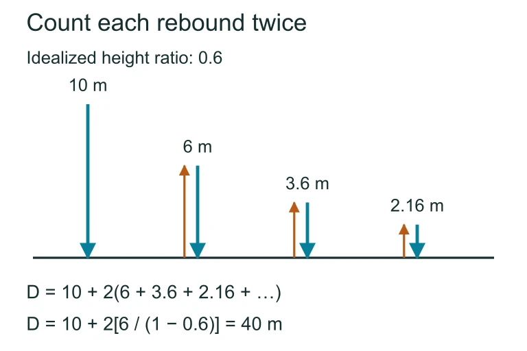A ball falls 10 m and rebounds to 60% of its preceding height. Count the initial fall once and each rebound twice: the geometric series gives 40 m of total travel.

SECTION 5

Detailed Technique Breakdown

The table below summarizes the main algebraic and calculus techniques for converting a function into a power series. Each technique is paired with a prototype function to illustrate when and how to apply it. Mastering this catalog is the most efficient way to handle AP exam problems, because nearly every question reduces to one of these patterns.

Technique	Prototype Function	Key Step	Result
Direct substitution	1/(1 + x²)	Replace u with −x² in 1/(1 − u)	Σ (−1)ⁿ x²ⁿ, \|x\| < 1
Factor & substitute	3/(2 + x)	Rewrite as (3/2)·1/(1 − (−x/2))	Σ (3/2)(−1)ⁿ(x/2)ⁿ, \|x\| < 2
Partial fractions	1/((1 − x)(1 + x))	Split into ½·1/(1 − x) + ½·1/(1 + x)	Σ ½(1 + (−1)ⁿ)xⁿ, \|x\| < 1
Term-by-term integration	ln(1 + x)	Integrate 1/(1 + x) = Σ (−1)ⁿ xⁿ	Σ (−1)ⁿ xⁿ⁺¹/(n + 1), \|x\| < 1
Term-by-term differentiation	1/(1 − x)²	Differentiate 1/(1 − x) = Σ xⁿ	Σ (n + 1)xⁿ, \|x\| < 1
Multiplication by x or xᵏ	x/(1 − x)	Multiply Σ xⁿ by x	Σ xⁿ⁺¹ = Σ xⁿ (n ≥ 1), \|x\| < 1

Catalog of power series conversion techniques tested on AP Calculus BC

Decision flowchart for converting f(x) into a power series. Start at the top and follow the branches: direct substitution is always the first check; if the function does not fit the 1/(1 − u) form, try factoring, partial fractions, or recognizing f as the integral or derivative of a simpler known series.

The flowchart above should become your mental checklist. When a problem says "represent f(x) as a power series," resist the urge to start computing Taylor coefficients via derivatives. Instead, ask: Can I rewrite f(x) so that it looks like a/(1 − u)? If the answer is yes—even after some algebra—you have a geometric series in disguise. If the answer is no, check whether f is the derivative or antiderivative of something that does fit. This systematic approach saves enormous time under exam pressure.

SECTION 6

Worked Example

Let us work through a complete problem of the type frequently seen on the AP Calculus BC exam. The task is to represent f(x) = 3x²/(1 + x³) as a power series centered at 0 and state the interval of convergence.

Represent f(x) = 3x² / (1 + x³) as a Power Series

1
Step 1 — Rewrite in geometric form

Observe that 1/(1 + x³) = 1/(1 − (−x³)). This matches the template 1/(1 − u) with u = −x³. The constant 3x² out front will multiply the entire series.
2
Step 2 — Expand using the geometric series

1/(1 − (−x³)) = Σ (−x³)ⁿ = Σ (−1)ⁿ x³ⁿ for n = 0 to ∞, provided |−x³| < 1, i.e., |x| < 1.
3
Step 3 — Multiply by the outside factor

f(x) = 3x² · Σ (−1)ⁿ x³ⁿ = Σ 3(−1)ⁿ x³ⁿ⁺² for n = 0 to ∞.

f(x) = Σ 3(−1)ⁿ x³ⁿ⁺²
4
Step 4 — Write the first few terms as a check

n = 0: 3x². n = 1: −3x⁵. n = 2: 3x⁸. n = 3: −3x¹¹. So f(x) = 3x² − 3x⁵ + 3x⁸ − 3x¹¹ + ⋯. You can verify: multiply this by (1 + x³) and all terms except 3x² cancel, confirming the identity.
5
Step 5 — State the interval of convergence

The convergence condition is |−x³| < 1, which simplifies to |x|³ < 1, i.e., |x| < 1. Check endpoints: at x = 1, the series becomes 3 − 3 + 3 − 3 + ⋯ (diverges). At x = −1, the series becomes 3 + 3 + 3 + ⋯ (diverges). Therefore the interval of convergence is (−1, 1).

Interval of convergence: (−1, 1)

ℹ

Observation

Notice something elegant: 3x²/(1 + x³) is exactly d/dx[ln(1 + x³)]. If the problem instead asked for the power series of ln(1 + x³), you would integrate the series we just found term by term. This interconnectedness is the real power of the technique.

SECTION 7

Strengths, Limitations & Comparisons

Representing functions as power series via the geometric series approach is one of two main strategies, the other being the formal Taylor/Maclaurin coefficient formula. Each has strengths and weaknesses, and the AP exam expects you to choose the right tool for the right problem. The table below contrasts the two approaches head to head.

Feature	Geometric Series Manipulation	Taylor/Maclaurin Coefficient Formula
Speed	Very fast for rational functions; no derivative computation needed	Slower; requires computing f⁽ⁿ⁾(c) for each term
Generality	Limited to functions expressible via 1/(1 − u) and its calculus relatives	Works for any infinitely differentiable function
Convergence info	Interval of convergence drops out naturally from \|u\| < 1	Requires a separate convergence test (ratio, root, etc.)
Error	Closed-form remainder via geometric series formula	Lagrange or alternating series error bound
Best for	Rational functions, integrals of rational functions, arctan, ln(1 ± x)	eˣ, sin x, cos x, and any function not reducible to geometric form

Comparison of the two primary power series construction methods

✦

KEY TAKEAWAY

Think of the geometric series method as your express lane and the Taylor coefficient formula as your local road. The express lane is faster but only goes certain places; the local road can reach any destination. On the AP exam, check the express lane first—if it applies, you save valuable minutes. If it doesn't, fall back to computing derivatives.

SECTION 8

Connection to Advanced Theory

The skill of representing functions as power series is not an end in itself—it is the gateway to several advanced techniques that appear both later in the AP curriculum and in college-level analysis. Understanding where this topic leads will help you appreciate why the College Board devotes significant weight to it.

This Lesson (Power Series via Geometric)	Advanced Extension
1/(1 − x) = Σ xⁿ with \|x\| < 1	Laurent series allow negative powers and represent functions with singularities in complex analysis
Term-by-term integration to find ln(1 + x)	Power series solutions to differential equations (Frobenius method) use term-by-term operations systematically
Interval of convergence from \|u\| < 1	Analytic continuation extends a power series beyond its natural radius using complex variable techniques
Partial fractions → separate geometric series	Generating functions in combinatorics encode sequences as power series coefficients for counting problems

From AP Calculus BC to college mathematics and beyond

On the AP exam itself, power series representations connect directly to Taylor polynomial approximations and Lagrange error bounds. Once you have a power series for f, truncating it gives a Taylor polynomial, and the remainder term tells you how close the approximation is. Free-response questions in Part B often chain these ideas: find a power series, use it to evaluate an integral, and then bound the error of a partial sum—all within a single multi-part problem.

SECTION 9

Practice Problems

Question 1: CONCEPTUAL

Which of the following best explains why the power series representation of 1/(1 + x) obtained by substituting u = −x into the geometric series 1/(1 − u) = Σ uⁿ is identical to the Maclaurin series obtained by computing f⁽ⁿ⁾(0)/n! for every n?

A. Because geometric series and Maclaurin series use the same convergence tests
B. Because 1/(1 + x) is a polynomial, so all representations are trivially the same
C. Because any two power series centered at the same point that converge to the same function on an interval must have identical coefficients (uniqueness of power series)
D. Because the ratio test always produces the same radius of convergence regardless of method
E. Because substitution into the geometric series is simply a shortcut notation for the Maclaurin derivative formula

Show answer (C)

The correct answer is C. The uniqueness theorem for power series states that if two power series centered at the same point converge to the same function on some interval, their coefficients must be identical. This is the deep reason why the geometric substitution method and the derivative-based Maclaurin method produce the same series. Choice A is wrong because convergence tests determine whether a series converges, not whether two convergent series must agree. Choice B is wrong because 1/(1 + x) is not a polynomial—it is a rational function with an infinite Maclaurin expansion. Choice D is incorrect because while the radius of convergence is the same, having the same radius does not by itself force coefficients to match. Choice E is tempting but misleading: the geometric substitution is not merely a notational shortcut for the derivative formula—it is a genuinely different computational path that arrives at the same result because of uniqueness.

Question 2: BASIC CALCULATION

Find the power series representation centered at 0 for f(x) = 5/(2 − x) and state the radius of convergence.

A. Σ (5/2)(x/2)ⁿ for n = 1 to ∞, R = 2
B. Σ (5/2)(x/2)ⁿ for n = 0 to ∞, R = 2
C. Σ 5(x/2)ⁿ for n = 0 to ∞, R = 2
D. Σ 5(−1)ⁿ(x/2)ⁿ for n = 0 to ∞, R = 2
E. Σ (5/2)(x/2)ⁿ for n = 0 to ∞, R = 1

Show answer (B)

The correct answer is B. Rewrite: 5/(2 − x) = (5/2) · 1/(1 − x/2). Apply the geometric series template 1/(1 − u) = Σ uⁿ with u = x/2: (5/2) · Σ (x/2)ⁿ = Σ (5/2)(x/2)ⁿ for n = 0 to ∞. Convergence requires |x/2| < 1, so |x| < 2 and R = 2. Choice A starts the summation at n = 1 instead of n = 0, which omits the constant term 5/2 and therefore represents 5/(2 − x) − 5/2 = 5x/(2(2 − x)), not the original function. Choice C is missing the factor of 1/2 out front—Σ 5(x/2)ⁿ = 5 · 1/(1 − x/2) = 10/(2 − x), which is twice the original function. Choice D incorrectly introduces (−1)ⁿ, which would apply if the denominator were (2 + x) instead of (2 − x). Choice E has the correct series but the wrong radius—R = 1 would apply if u were x instead of x/2.

Question 3: INTERMEDIATE

Find the power series representation for f(x) = arctan(x) centered at 0 by integrating the power series for 1/(1 + x²). Express the general term and state the radius of convergence.

A. Σ (−1)ⁿ x²ⁿ⁺¹/(2n + 1) for n = 0 to ∞, R = 1
B. Σ (−1)ⁿ x²ⁿ/(2n) for n = 1 to ∞, R = 1
C. Σ (−1)ⁿ x²ⁿ⁺¹/(2n + 1) for n = 0 to ∞, R = ∞
D. Σ x²ⁿ⁺¹/(2n + 1) for n = 0 to ∞, R = 1
E. Σ (−1)ⁿ x²ⁿ⁺²/(2n + 2) for n = 0 to ∞, R = 1

Show answer (A)

The correct answer is A. Begin with 1/(1 + x²) = 1/(1 − (−x²)) = Σ (−1)ⁿ x²ⁿ for |x| < 1. Since d/dx[arctan x] = 1/(1 + x²), integrate term by term: arctan x = C + Σ (−1)ⁿ x²ⁿ⁺¹/(2n + 1). Setting x = 0 gives arctan 0 = 0, so C = 0. The radius of convergence is R = 1, inherited from the geometric series condition |x²| < 1. Choice B has the wrong exponents and denominators—it attempts to integrate incorrectly. Choice C has the right series but claims R = ∞, which is false; arctan x is defined for all x, but the power series only converges for |x| ≤ 1. Choice D omits the alternating sign (−1)ⁿ. Choice E integrates incorrectly, producing even powers x²ⁿ⁺² instead of odd powers x²ⁿ⁺¹.

Question 4: APPLIED

5 pts

A physics model requires evaluating the integral ∫₀^(0.5) x²/(1 + x⁴) dx. Use a power series representation to express this integral as an infinite series, then compute an approximation using the first three nonzero terms. Show all steps, including how you obtain the power series, perform the term-by-term integration, and evaluate the resulting series at the bounds.

Show answer

Point 1 (Power series setup — 1 pt): Recognize that 1/(1 + x⁴) = 1/(1 − (−x⁴)) = Σ (−1)ⁿ x⁴ⁿ for |x| < 1. Since 0.5 < 1, the interval is valid. Point 2 (Multiply and write integrand series — 1 pt): x²/(1 + x⁴) = x² · Σ (−1)ⁿ x⁴ⁿ = Σ (−1)ⁿ x⁴ⁿ⁺² for n = 0 to ∞. Point 3 (Term-by-term integration — 1 pt): ∫₀^(0.5) Σ (−1)ⁿ x⁴ⁿ⁺² dx = Σ (−1)ⁿ [x⁴ⁿ⁺³/(4n + 3)] from 0 to 0.5 = Σ (−1)ⁿ (0.5)⁴ⁿ⁺³/(4n + 3). Point 4 (Evaluate first three terms — 1 pt): n = 0: (0.5)³/3 = 0.125/3 ≈ 0.041667. n = 1: −(0.5)⁷/7 = −0.0078125/7 ≈ −0.001116. n = 2: (0.5)¹¹/11 = 0.000488281/11 ≈ 0.0000444. Point 5 (Sum and conclude — 1 pt): Approximate value ≈ 0.041667 − 0.001116 + 0.000044 ≈ 0.040595. Since this is an alternating series with decreasing terms, the error is bounded by the absolute value of the first omitted term, which is (0.5)¹⁵/15 ≈ 0.00000204, so the three-term approximation is accurate to about five decimal places.

Question 5: CRITICAL THINKING

3 pts

The function g(x) = x/(1 − x)² can be expressed as a power series by differentiating the geometric series. Derive the power series for g(x) centered at 0, state the radius of convergence, and explain why this particular derivation works even though g has a second-order pole at x = 1.

Show answer

Point 1 (Derivation — 1 pt): Start with 1/(1 − x) = Σ xⁿ for |x| < 1. Differentiate both sides: 1/(1 − x)² = Σ n·xⁿ⁻¹ = Σ (n + 1)xⁿ for n = 0 to ∞. Multiply by x: g(x) = x/(1 − x)² = Σ (n + 1)xⁿ⁺¹ = Σ n·xⁿ for n = 1 to ∞. Point 2 (Radius of convergence — 1 pt): Term-by-term differentiation preserves the open interval of convergence. Since the original geometric series has R = 1, the differentiated series also has R = 1, convergent for |x| < 1. Point 3 (Explanation of the pole — 1 pt): A second-order pole at x = 1 means g(x) → ∞ as x → 1. This does not invalidate the power series representation because the series is only claimed to represent g on |x| < 1, which excludes the singularity. The radius of convergence R = 1 is precisely determined by the distance from the center (x = 0) to the nearest singularity (x = 1), which is consistent with the general theorem that a power series converges up to (but not including) the nearest singularity in the complex plane.

SUMMARY

Summary — Representing Series as Power Series

Summary

Representing a function as a power series centers on the geometric series template 1/(1 − u) = Σ uⁿ, which converges for |u| < 1. By rewriting a target function into this form via algebraic manipulation—including factoring, substitution, and partial fraction decomposition—you can express a wide class of rational functions as power series without computing any derivatives. The interval of convergence emerges naturally from the condition |u| < 1, and endpoints must always be checked separately.

Two calculus-based extensions—term-by-term differentiation and term-by-term integration—let you build series for functions like arctan x, ln(1 + x), and 1/(1 − x)² from the foundational geometric series. The uniqueness of power series representations guarantees that every valid method—whether geometric manipulation or the Taylor coefficient formula—produces the same result, giving you confidence to use whichever approach is fastest for the problem at hand.