Rates of Change in Applied Concepts Other Than Motion - AP Calculus BC

SECTION 1

Historical Context & Motivation

When Newton and Leibniz formalized calculus in the late seventeenth century, the prototypical application was motion — velocity as the derivative of position, acceleration as the derivative of velocity. Yet within a generation, mathematicians and scientists recognized that the same machinery could describe the rate at which any measurable quantity changes with respect to an independent variable. Heat transfer, population dynamics, chemical concentrations, economic output — all of these processes involve quantities whose instantaneous rates of change carry deep physical or contextual meaning. The story of how differentiation escaped the physics classroom and permeated every quantitative discipline illuminates why the AP Calculus BC curriculum devotes an entire topic to interpreting derivatives in non-motion contexts.

1687 • Newton's Principia

Isaac Newton publishes the Principia Mathematica, framing derivatives ("fluxions") primarily in terms of motion and gravitational mechanics.

1736 • Euler's Mechanica

Leonhard Euler extends differential methods to fluid flow and elasticity, demonstrating that rates of change apply far beyond particle kinematics.

1822 • Fourier's Théorie Analytique de la Chaleur

Joseph Fourier models heat conduction using differential equations, showing that temperature changes over time are governed by derivatives — a landmark non-motion application.

1838 • Verhulst's Logistic Growth Model

Pierre-François Verhulst models population growth with a differential equation dP/dt = rP(1 − P/K), making population ecology a calculus-based science.

1890s • Marginal Analysis in Economics

Alfred Marshall and the marginalist economists define marginal cost and marginal revenue as derivatives, embedding calculus at the heart of microeconomic theory.

The central question this topic addresses is deceptively simple: if a quantity Q depends on a variable t (which need not be time), what does dQ/dt tell us about the real-world process? On the AP exam, you will be asked to interpret the sign, magnitude, and units of a derivative in context — and to distinguish between average and instantaneous rates of change when neither quantity involves position or velocity.

SECTION 2

Core Principles & Definitions

Before diving into specific applications, it is essential to internalize the handful of foundational ideas that govern every rates-of-change problem you will encounter on the exam. The derivative is a single mathematical object, but its contextual meaning shifts dramatically depending on what Q and t represent.

Instantaneous Rate of Change

If Q(t) is a differentiable function, then dQ/dt at t = a gives the instantaneous rate at which Q changes per unit of the independent variable at that specific moment. This is the slope of the tangent line to Q at t = a.

Average Rate of Change

Over an interval [a, b], the average rate of change is ΔQ/Δt = (Q(b) − Q(a))/(b − a). This is the slope of the secant line and serves as a discrete approximation to the derivative when only tabular data are available.

Units of the Derivative

The units of dQ/dt are always [units of Q] per [unit of t]. If Q is measured in gallons and t in minutes, then dQ/dt has units of gallons per minute. Correct unit interpretation is tested on every AP exam.

Sign Interpretation

A positive derivative means Q is increasing; a negative derivative means Q is decreasing; a zero derivative indicates a local extremum or an inflection point (if the concavity also changes). In context, the sign tells you the direction of the process.

Second Derivative as Rate of a Rate

d²Q/dt² describes how the rate of change itself is changing. In economics, if marginal cost is increasing, d²C/dq² > 0; in biology, if a population's growth rate is slowing, d²P/dt² < 0.

✦

KEY TAKEAWAY

Think of the derivative as a universal "speedometer" — but instead of measuring miles per hour, it measures anything per anything. A chemical engineer reads dC/dt like a speedometer for concentration change; an economist reads dR/dq like a speedometer for revenue generated by the next unit sold. The calculus is identical; only the labels on the dial change.

SECTION 3

Visual Explanation — Interpreting Derivatives Graphically

The diagram below shows a generic quantity Q(t) — it could represent the temperature of a cooling object, the volume of water in a tank, or the amount of a drug in a patient's bloodstream. The tangent line at t = a has slope equal to dQ/dt|₍ₜ₌ₐ₎, while the secant line from t = a to t = b has slope equal to the average rate of change over [a, b]. Observe how the tangent line captures the behavior at a single instant, whereas the secant line averages over the entire interval.

The cyan tangent line at t = a has slope dQ/dt, representing the instantaneous rate of change. The pink secant line connecting (a, Q(a)) and (b, Q(b)) has slope ΔQ/Δt, representing the average rate of change over [a, b].

Notice that wherever Q(t) is concave up (the curve bends upward), the instantaneous rate of change is increasing — the tangent line gets steeper as t advances. This means d²Q/dt² > 0 in that region. Conversely, where Q(t) is concave down, the tangent slope is decreasing and d²Q/dt² < 0. On the AP exam, you may be asked to read the sign of the first or second derivative from a graph and interpret it in the given context: "the temperature is decreasing at a decreasing rate" means dT/dt < 0 and d²T/dt² > 0, because the rate of temperature drop is becoming less severe.

SECTION 4

Mathematical Framework

The formal definitions underlying rates of change in applied contexts are straightforward extensions of the limit definition of the derivative. What distinguishes applied-rate problems from pure differentiation exercises is the need to attach correct units and contextual interpretations to every symbolic expression.

AVERAGE RATE OF CHANGE

Average rate = ΔQ / Δt = [Q(b) − Q(a)] / (b − a)

Q is the dependent quantity (e.g., temperature, cost, population), and t is the independent variable (e.g., time, production level, distance). The result carries units of [Q-units] per [t-unit].

INSTANTANEOUS RATE OF CHANGE

dQ/dt = lim (Δt → 0) [Q(t + Δt) − Q(t)] / Δt

This limit, when it exists, gives the exact rate at a single value of t. On the AP exam, you are often given Q(t) as a formula and asked to evaluate dQ/dt at a particular t, then interpret the answer.

SECOND DERIVATIVE INTERPRETATION

d²Q/dt² = d/dt [dQ/dt]

Positive d²Q/dt² means the rate of change is increasing (the process is accelerating in the Q-direction). Negative d²Q/dt² means the rate of change is decreasing (the process is decelerating). This is analogous to acceleration in motion but applies to any context.

MARGINAL ANALYSIS (ECONOMICS)

C′(q) = dC/dq ≈ C(q + 1) − C(q)

In economics, the derivative of the cost function C(q) with respect to quantity q gives the marginal cost — the approximate cost of producing one additional unit. Similarly, R′(q) = dR/dq is marginal revenue. Profit is maximized where R′(q) = C′(q).

💡

AP EXAM TIP

Free-response questions frequently present data in a table rather than a formula. When no closed-form expression for Q(t) is given, you must estimate the derivative using the average rate of change over the smallest available interval: dQ/dt|₍ₜ₌ₐ₎ ≈ [Q(a + h) − Q(a − h)] / (2h), where h is the half-width of the table's surrounding entries. Always include units in your answer.

SECTION 5

Application Domains — A Classification

While the underlying calculus is identical across domains, the AP exam draws from several distinct real-world contexts. Familiarity with each context — its typical variables, its units, and the physical or economic meaning of the derivative — will save precious time on test day. The diagram below organizes the most common non-motion application categories, and the table that follows provides concrete details for each.

A taxonomy of non-motion rate-of-change contexts commonly tested on the AP Calculus BC exam, organized by domain. Each leaf node shows the derivative notation and its units.

Context	Q (dependent)	t (independent)	dQ/dt meaning	Typical units
Temperature (cooling)	T — temperature	t — time	How fast the object is cooling or heating	°C/min or °F/hr
Tank / fluid volume	V — volume of fluid	t — time	Rate of filling or draining	gal/min or L/s
Economics — cost	C — total cost	q — quantity produced	Marginal cost: additional cost per unit	$/unit
Population biology	P — population size	t — time	Growth or decline rate	organisms/year
Charge / current	Q — electric charge	t — time	Electric current I = dQ/dt	coulombs/sec = amperes

Common non-motion contexts for derivatives on the AP Calculus BC exam

SECTION 6

Worked Example — Cost Function & Marginal Analysis

A manufacturer's total cost (in dollars) for producing q units of a product is modeled by C(q) = 0.004q³ − 0.6q² + 35q + 800. Find and interpret the marginal cost when q = 50 units, and determine whether the marginal cost is increasing or decreasing at that production level.

Marginal Cost Analysis

1
Step 1 — Identify the derivative's meaning

The marginal cost is defined as C′(q) = dC/dq. This represents the approximate additional cost, in dollars, incurred by producing one more unit when q units have already been produced.
2
Step 2 — Differentiate C(q)

C′(q) = d/dq [0.004q³ − 0.6q² + 35q + 800] = 0.012q² − 1.2q + 35. Note that the constant term 800 (fixed costs) vanishes upon differentiation — fixed costs do not affect marginal cost.

C′(q) = 0.012q² − 1.2q + 35
3
Step 3 — Evaluate at q = 50

C′(50) = 0.012(50)² − 1.2(50) + 35 = 0.012(2500) − 60 + 35 = 30 − 60 + 35 = 5.

C′(50) = $5 per unit
4
Step 4 — Interpret in context

When the company is already producing 50 units, the cost of producing the 51st unit is approximately $5. This is a relatively low marginal cost, suggesting that the production level is in an efficient range.
5
Step 5 — Second derivative for concavity

C″(q) = d/dq [0.012q² − 1.2q + 35] = 0.024q − 1.2. At q = 50: C″(50) = 0.024(50) − 1.2 = 1.2 − 1.2 = 0. Since C″(50) = 0, the marginal cost is at a transition point. For q < 50, C″(q) < 0 (marginal cost decreasing — economies of scale). For q > 50, C″(q) > 0 (marginal cost increasing — diseconomies of scale). Therefore q = 50 is the production level at which marginal cost is minimized.

C″(50) = 0 → marginal cost is minimized at q = 50

SECTION 7

Common Pitfalls & Exam Strategies

Understanding the calculus is only half the battle — the other half is communicating your answer with the precision the AP graders expect. The table below contrasts common mistakes with the corresponding correct approaches, covering errors that appear with alarming frequency on free-response questions involving applied rates of change.

Common Pitfall	Why It's Wrong	Correct Approach
Omitting units from the derivative	The derivative's meaning is inseparable from its units. A numerical answer without units earns no interpretation credit.	Always write dQ/dt = [value] [Q-units per t-unit] and state the interpretation in a complete sentence.
Confusing average and instantaneous rates	ΔQ/Δt from a table is an average rate over an interval, not the exact derivative at a point.	Use language such as "approximates the rate" when using table data; use "equals" only when computing the exact derivative from a formula.
Ignoring the sign of the derivative	A negative derivative is not an error — it means Q is decreasing. Reporting \|dQ/dt\| loses directional information.	State whether Q is increasing or decreasing and tie the sign back to the physical context.
Misinterpreting the second derivative	"d²Q/dt² > 0 means Q is increasing" is false — it means the rate of change is increasing.	A positive second derivative says the first derivative is increasing (concave up). Q itself may still be decreasing if dQ/dt < 0.
Using a tangent-line approximation far from the point of tangency	Linearization is only accurate near the point of tangency; extrapolating far introduces large errors, especially when the function is concave.	Use the approximation Q(a + h) ≈ Q(a) + Q′(a)·h only for small h. If asked about accuracy, note the sign of d²Q/dt² (overestimate vs. underestimate).

Common exam pitfalls in applied rate-of-change problems

✦

KEY TAKEAWAY

The AP graders are evaluating your ability to translate between calculus and context. Think of yourself as a bilingual interpreter: fluent in the language of mathematics (dQ/dt, concavity, limits) and equally fluent in the language of the given scenario (gallons per minute, dollars per unit, organisms per year). The exam rewards those who bridge both languages in every sentence of their response.

SECTION 8

Connections to Advanced Topics

The applied rate-of-change framework developed in this lesson is not an isolated topic — it is the conceptual foundation for several more advanced areas of the AP Calculus BC curriculum. Understanding how derivatives operate in non-motion contexts prepares you for related rates (where multiple applied quantities change simultaneously), for differential equations (where the rate of change is related to the quantity itself), and for the Fundamental Theorem of Calculus applied in context (where accumulation functions arise from rate functions).

This Lesson (Applied Rates)	Advanced Extension
dQ/dt interpreted in a single context	Related Rates: multiple dQ/dt's linked by an equation (e.g., dV/dt and dr/dt for a balloon)
Marginal cost C′(q) and marginal revenue R′(q)	Optimization: find q where profit P(q) = R(q) − C(q) is maximized, using P′(q) = 0 and P″(q) < 0
dP/dt = rP (exponential growth rate)	Differential Equations: dP/dt = rP(1 − P/K) logistic growth, separation of variables, slope fields
Average rate ΔQ/Δt over [a, b]	Mean Value Theorem: guarantees existence of c in (a, b) with Q′(c) = ΔQ/Δt
Rate function R(t) describes flow into a tank	Accumulation: Total volume = ∫₀ᵀ R(t) dt via the Fundamental Theorem of Calculus

How applied rate-of-change ideas extend to later BC topics

As you progress through the course, you will notice that nearly every new topic asks you to do something with a derivative (or an integral) in context. The skills you build here — identifying units, interpreting signs, and distinguishing average from instantaneous rates — are not one-time tools but recurring competencies that the exam assesses throughout all six free-response questions and across multiple-choice items.

A stirred transparent tank has one upper inlet and one lower outlet with a valve. The exact diagram links its 100 L salt balance to a computed approach to equilibrium. Suppose a tank receives and releases 4 gal/min for 5 minutes. Its 200 gal inventory stays constant while 20 gal enters and 20 gal leaves: net change is zero and total throughput is 40 gal.

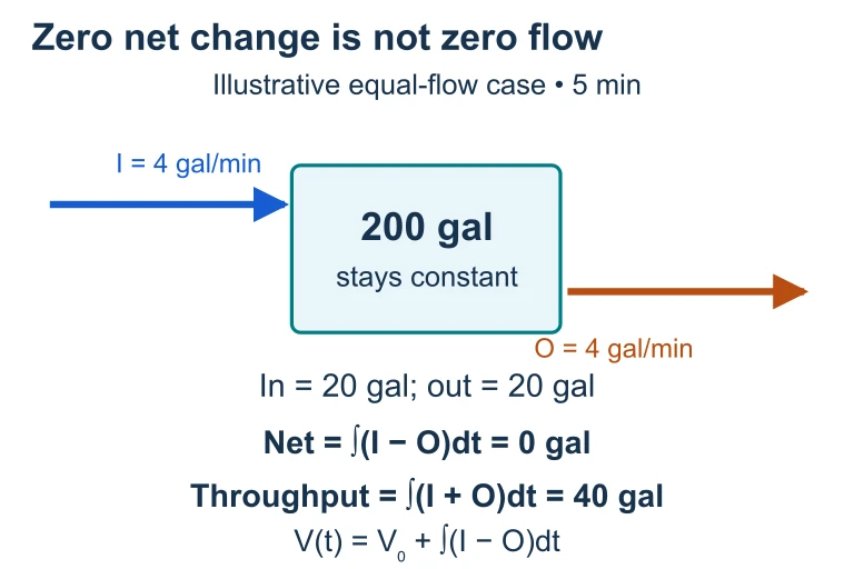Suppose a tank receives and releases 4 gal/min for 5 minutes. Its 200 gal inventory stays constant while 20 gal enters and 20 gal leaves: net change is zero and total throughput is 40 gal.

SECTION 9

Practice Problems

Question 1: CONCEPTUAL

The temperature T(t) of a cup of coffee is measured in degrees Fahrenheit, and t is measured in minutes after the coffee is poured. If T′(5) = −3.2, which of the following is the best interpretation?

A. At t = 5 minutes, the coffee's temperature is −3.2 °F.
B. At t = 5 minutes, the coffee's temperature is decreasing at a rate of 3.2 °F per minute.
C. Over the first 5 minutes, the coffee's temperature decreased by a total of 3.2 °F.
D. At t = 5 minutes, the coffee's temperature is increasing at a rate of 3.2 °F per minute.
E. The coffee reaches its minimum temperature at t = 5 minutes.

Show answer (B)

B is correct. T′(5) = −3.2 means the instantaneous rate of change of temperature at t = 5 is −3.2 °F/min, so the temperature is decreasing at 3.2 °F per minute. A is wrong because T′(5) is the rate of change, not the temperature itself. C is wrong because T′(5) gives an instantaneous rate, not a total change over 5 minutes (that would be T(5) − T(0)). D is wrong because the negative sign means the temperature is decreasing, not increasing. E is wrong because T′(5) = −3.2 ≠ 0; a minimum would require T′ = 0.

Question 2: BASIC CALCULATION

A company's revenue function is R(q) = 120q − 0.5q², where R is in dollars and q is the number of units sold. What is the marginal revenue when q = 80 units?

A. $40 per unit
B. $80 per unit
C. $6400
D. $120 per unit
E. −$40 per unit

Show answer (A)

A is correct. R′(q) = 120 − q, so R′(80) = 120 − 80 = 40 dollars per unit. B ($80) is simply the value of q, not the marginal revenue. C ($6400) is R(80) = 120(80) − 0.5(80)² = 9600 − 3200 = 6400, the total revenue rather than the marginal revenue. D ($120) is R′(0), the marginal revenue at zero production, not at q = 80. E (−$40) incorrectly negates the result; the derivative is positive at q = 80 because q < 120.

Question 3: INTERMEDIATE

The number of bacteria in a culture at time t hours is modeled by N(t) =

2000e^{0.15t}

. At what rate is the population growing when there are exactly 5000 bacteria in the culture?

A. 300 bacteria per hour
B. 500 bacteria per hour
C. 750 bacteria per hour
D. 916 bacteria per hour
E. 1000 bacteria per hour

Show answer (C)

C is correct. N′(t) = 2000 × 0.15 ×

e^{0.15t}

300e^{0.15t}

. Equivalently, N′(t) = 0.15 × N(t). When N = 5000, the rate is N′ = 0.15 × 5000 = 750 bacteria per hour. A (300) is N′(0) = 0.15 × 2000, the rate at t = 0 when the population is 2000, not 5000. B (500) is 5000/10 or a common arithmetic error. D (916) results from first solving for t = ln(2.5)/0.15 ≈ 6.11 and then making a rounding error. E (1000) may arise from the misconception that the rate is 0.2N rather than 0.15N.

Question 4: APPLIED

5 pts

A tank initially holds 200 gallons of water. Water flows into the tank at a rate of F(t) = 10 + 2sin(t²) gallons per minute and drains out at a constant rate of 8 gallons per minute for 0 ≤ t ≤ 5 minutes. (a) Write an expression for the rate of change of the volume of water in the tank at time t. (b) Is the volume of water in the tank increasing or decreasing at t = 2 minutes? Justify your answer. (c) At what time t, for 0 < t < 5, does the volume of water in the tank reach its maximum? Justify your reasoning. (d) Write, but do not evaluate, an integral expression for the total volume of water in the tank at t = 5 minutes.

Show answer

Point-by-point rubric: (a) [1 point] dV/dt = F(t) − 8 = 10 + 2sin(t²) − 8 = 2 + 2sin(t²) gallons per minute. Award 1 point for the correct net-rate expression with correct units. (b) [1 point] At t = 2, dV/dt = 2 + 2sin(4). Since sin(4) ≈ −0.7568, dV/dt ≈ 2 + 2(−0.7568) = 2 − 1.5136 = 0.4864 > 0. Because dV/dt > 0 at t = 2, the volume is increasing at t = 2 minutes. Award 1 point for correct evaluation, correct sign conclusion, and interpretation in context. (c) [2 points] The volume is maximized when dV/dt changes from positive to negative. Set dV/dt = 0: 2 + 2sin(t²) = 0 → sin(t²) = −1 → t² = 3π/2 → t = √(3π/2) ≈ 2.171. We verify this is a maximum: for t slightly less than √(3π/2), sin(t²) > −1 so dV/dt > 0; for t slightly greater, sin(t²) < −1 is impossible, so we examine that sin(t²) increases past −1, meaning dV/dt becomes positive again. Alternatively, use the first derivative test or evaluate d²V/dt² at the critical point. [1 point for finding the correct critical value; 1 point for justification via sign change or second derivative test.] (d) [1 point] V(5) = 200 + ∫₀⁵ [2 + 2sin(t²)] dt. Award 1 point for the correct initial value plus the correct definite integral of the net rate function.

Question 5: CRITICAL THINKING

3 pts

Let P(t) represent the profit, in thousands of dollars, earned by a company t months after launching a new product. The table below gives selected values of P′(t). t (months): 0 3 6 9 12 P′(t) (thousands of $/month): 8 5 1 −2 −4 (a) Estimate P″(6) using values from the table. Show your computation and include units. (b) Using your answer from (a), interpret P″(6) in the context of the problem. (c) Based on the data, is there a time t in the interval (0, 12) at which P′(t) = 0? Justify your answer using a theorem from calculus.

Show answer

Point-by-point rubric: (a) [1 point] Using a symmetric difference quotient: P″(6) ≈ [P′(9) − P′(3)] / (9 − 3) = (−2 − 5) / 6 = −7/6 ≈ −1.167 thousands of dollars per month per month, i.e., approximately −1167 dollars/month². Award 1 point for the correct quotient with correct units. (b) [1 point] At t = 6 months, the rate of profit growth is decreasing at approximately 1.167 thousand dollars per month per month. In context, although the company is still earning profit at a positive rate at t = 6 (since P′(6) = 1 > 0), the profitability is decelerating — each successive month brings less additional profit than the previous month. Award 1 point for a correct contextual interpretation that references the rate of the rate (or how the profit growth rate is changing). (c) [1 point] Yes. Since P′ is continuous (assuming P is twice-differentiable), and P′(6) = 1 > 0 while P′(9) = −2 < 0, by the Intermediate Value Theorem there exists at least one time c in (6, 9) ⊂ (0, 12) such that P′(c) = 0. At this time, the profit has a critical point — a likely maximum. Award 1 point for correctly citing the IVT, verifying its hypotheses (continuity and a sign change), and reaching the correct conclusion.

SUMMARY

Lesson Summary

Summary

The derivative dQ/dt measures the instantaneous rate of change of any quantity Q with respect to an independent variable t, carrying units of [Q-units] per [t-unit]. Whether Q represents temperature, cost, population, volume, or concentration, the calculus is identical: differentiate, evaluate, and interpret the sign and magnitude in context. A positive derivative means Q is increasing, a negative derivative means Q is decreasing, and the second derivative d²Q/dt² reveals whether the rate of change is itself increasing or decreasing.

On the AP exam, success requires more than computation: you must state units with every derivative value, distinguish average from instantaneous rates (especially when working from tables), use the Intermediate Value Theorem to justify the existence of critical points, and write complete contextual sentences that translate mathematical results into real-world meaning. These skills form the bedrock for related rates, optimization, differential equations, and accumulation problems throughout the rest of the course.