Modeling Situations with Differential Equations - AP Calculus BC

SECTION 1

Historical Context & Motivation

The story of differential equations is inseparable from the birth of calculus itself. When Isaac Newton sought to describe the motion of planets and the cooling of heated objects, he recognized that the language of instantaneous rates of change was far more natural than static algebraic relationships. Rather than asking "where is the planet now?" Newton asked "how fast is the planet's position changing, and how does that rate depend on its current state?" This shift from static description to dynamic modeling through rates of change became one of the most powerful intellectual tools in the history of science, giving rise to an entire branch of mathematics devoted to equations involving derivatives.

1687 • Newton's Principia

Isaac Newton published the Principia Mathematica, formulating the laws of motion as differential equations relating force, mass, and acceleration—launching mathematical physics.

1736 • Euler's Systematic Methods

Leonhard Euler developed general techniques for solving ordinary differential equations, including the exponential function as the natural solution to dy/dx = ky, and introduced numerical approximation methods.

1798 • Malthus and Population Growth

Thomas Malthus proposed that population grows proportionally to its current size—an insight later modeled by the differential equation dP/dt = kP, one of the simplest and most important models in biology and economics.

1838 • Verhulst's Logistic Model

Pierre-François Verhulst refined Malthus's model by introducing a carrying capacity, yielding the logistic differential equation dP/dt = kP(1 − P/L). This equation realistically models bounded population growth and remains central to ecology.

1900s • Modern Applications Expand

Differential equation models became indispensable in engineering, pharmacokinetics, epidemiology (the SIR model), economics, and climate science—anywhere a system's future state depends on its present rate of change.

The central question that differential equations address is deceptively simple: if you know the rule governing how a quantity changes, can you determine the quantity itself? In AP Calculus BC, you will learn to translate verbal descriptions of rates of change into differential equations, classify the type of model involved, and solve or analyze these equations to make predictions about real-world phenomena.

SECTION 2

Core Principles & Definitions

Before diving into specific models, it is essential to establish what a differential equation is and the conceptual vocabulary that surrounds it. A differential equation is any equation that relates a function to one or more of its derivatives. In the context of AP Calculus BC, we focus exclusively on ordinary differential equations (ODEs) involving a single independent variable—typically time. The process of modeling involves three stages: translating a verbal or physical scenario into a differential equation, solving or analyzing the equation, and interpreting the solution in context.

Differential Equation

An equation relating an unknown function y(t) to its derivatives (dy/dt, d²y/dt², …). In BC, we focus on first-order ODEs of the form dy/dt = f(t, y).

Initial Condition

A known value of the function at a specific input, such as y(0) = 5. This pins down one particular solution from the family of all possible solutions.

General vs. Particular Solution

The general solution contains an arbitrary constant C representing all antiderivatives. Applying an initial condition yields the particular solution specific to the given scenario.

Proportionality Modeling

"The rate of change of y is proportional to y" translates to dy/dt = ky. Identifying proportionality statements in word problems is the key modeling skill on the AP exam.

Equilibrium Solutions

Constant values y₀ where dy/dt = 0 for all t. These solutions represent steady states—values toward which (or away from which) other solutions tend over time.

✦

KEY TAKEAWAY

Think of a differential equation as a recipe rather than a finished dish. The equation dy/dt = 2y tells you the rule for how y changes at every moment—like a GPS telling you your speed based on your current location. The solution y(t) is the actual route you travel. The initial condition is your starting address. Without the recipe (the DE), you cannot navigate; without the starting address (the IC), you don't know which route is yours among the infinitely many possibilities.

SECTION 3

Visual Explanation — From Words to Equations

The most critical skill tested on the AP Calculus BC exam is the ability to translate a verbal description of a rate of change into a precise differential equation. The diagram below illustrates the modeling pipeline: a real-world scenario is described in words, key phrases are identified and converted to mathematical expressions involving derivatives, and the resulting differential equation is classified by type. Understanding this process prevents the common error of confusing the rate of change dy/dt with the quantity y itself.

The modeling pipeline converts verbal statements about rates into differential equations. The key phrase translations in the lower section should be memorized—they appear repeatedly on the AP exam in both multiple-choice and free-response questions.

Notice that the phrase "rate of change" always indicates the presence of a derivative on the left side of the equation. The phrase "proportional to" introduces a proportionality constant k (which may be positive for growth or negative for decay). When the rate depends on the difference between the current value and some constant, you are typically looking at a Newton's Law of Cooling type model. When the rate depends on the product of y and (L − y), you have the logistic model. Being able to quickly classify a word problem into one of these types is the single most important skill in this topic.

SECTION 4

Mathematical Framework

AP Calculus BC focuses on three primary differential equation models, each arising from a distinct verbal pattern. Understanding the structure of these equations—how the right-hand side depends on the unknown function—determines both the qualitative behavior of solutions and the technique needed to solve them. All three are separable first-order ODEs, which means they can be solved by the method of separation of variables.

EXPONENTIAL GROWTH / DECAY

dy/dt = ky

Solution: y(t) = y₀e^kt, where y₀ = y(0). If k > 0, the quantity grows without bound; if k < 0, it decays toward zero. The rate of change is directly proportional to the current value of y.

LOGISTIC GROWTH

dy/dt = ky(1 − y/L)

Solution: y(t) = L / (1 + Ae^−kt), where A = (L − y₀)/y₀. Here L is the carrying capacity—the maximum sustainable population. The growth rate is fastest at y = L/2 (the inflection point) and slows as y approaches L.

NEWTON'S LAW OF COOLING

dT/dt = k(T − Tₑ)

Solution: T(t) = Tₑ + (T₀ − Tₑ)e^kt, where Tₑ is the ambient (environmental) temperature, T₀ = T(0) is the initial temperature, and k < 0. The rate of temperature change is proportional to the difference between the object's temperature and its surroundings.

GENERAL FIRST-ORDER SEPARABLE FORM

dy/dt = g(t) · h(y)

Any first-order ODE where the right side factors into a function of t alone times a function of y alone is separable. Rewrite as (1/h(y)) dy = g(t) dt and integrate both sides. All three models above are special cases of this form.

💡

AP Exam Tip

Free-response questions frequently ask you to write a differential equation from a verbal description without solving it. Earn full credit by correctly identifying the dependent variable, the independent variable, and the proportionality structure. Include the constant k even if its numerical value is not given.

SECTION 5

Classifying Models — A Visual Comparison

One of the most efficient strategies for the AP exam is to recognize which model applies based on the shape of the solution curve. Exponential growth produces a J-shaped curve that accelerates without bound; exponential decay produces a curve that asymptotically approaches zero. The logistic model produces an S-shaped (sigmoid) curve bounded by the carrying capacity L, with an inflection point at y = L/2. Newton's Law of Cooling produces a curve that asymptotically approaches the ambient temperature Tₑ. The diagram below compares all three solution behaviors on a single set of axes.

Three fundamental solution types compared: the pink curve shows unbounded exponential growth (J-shape), the green curve shows logistic growth (S-shape bounded by L with inflection at L/2), and the cyan curve shows exponential decay toward an equilibrium (the ambient temperature Tₑ). Recognizing these shapes on slope fields or from verbal descriptions is essential for the AP exam.

Feature	Exponential	Logistic	Newton's Cooling
DE Form	dy/dt = ky	dy/dt = ky(1 − y/L)	dT/dt = k(T − Tₑ)
Curve Shape	J-shaped (unbounded)	S-shaped (sigmoid)	Asymptotic decay
Equilibrium	y = 0 (unstable)	y = 0 (unstable), y = L (stable)	T = Tₑ (stable)
Key Verbal Cue	"proportional to itself"	"proportional to y and (L − y)"	"proportional to the difference"
Inflection Point	None	y = L/2	None

Comparison of the three fundamental differential equation models tested on AP Calculus BC

A steaming coffee cup and a cool liquid cup with condensation, each probed, with a shared room-reference probe between them. With ambient temperature 22 °C and k > 0, T′ = −k(T − 22). A warmer liquid cools and a cooler liquid warms, both approaching ambient temperature.

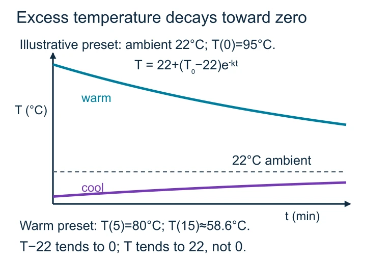With ambient temperature 22 °C and k > 0, T′ = −k(T − 22). A warmer liquid cools and a cooler liquid warms, both approaching ambient temperature.

SECTION 6

Worked Example — Modeling and Solving a Logistic Equation

A biologist introduces 200 fish into a lake that can sustain a maximum of 5000 fish. The fish population P(t) grows at a rate proportional to both the current population and the fraction of the carrying capacity still available. After 6 months, the population has grown to 800 fish. Write a differential equation modeling this situation, find the proportionality constant, and determine the population after 18 months.

Logistic Growth: Fish Population

1
Step 1 — Translate the verbal description into a DE

"Rate proportional to the current population and the fraction of carrying capacity still available" means dP/dt is proportional to P × (1 − P/L). With L = 5000, the differential equation is:

dP/dt = kP(1 − P/5000)
2
Step 2 — Write the general logistic solution

The general solution to the logistic equation dP/dt = kP(1 − P/L) is P(t) = L / (1 + Ae⁻ᵏᵗ). Using our values: P(t) = 5000 / (1 + Ae⁻ᵏᵗ). Now apply the initial condition P(0) = 200 to find A.

200 = 5000 / (1 + A) → 1 + A = 25 → A = 24
3
Step 3 — Use the second data point to find k

At t = 6 months, P(6) = 800. Substitute into the particular solution: 800 = 5000 / (1 + 24e⁻⁶ᵏ). Solving: 1 + 24e⁻⁶ᵏ = 5000/800 = 6.25, so 24e⁻⁶ᵏ = 5.25, giving e⁻⁶ᵏ = 5.25/24 = 0.21875. Take the natural log: −6k = ln(0.21875) ≈ −1.5198, so k ≈ 0.2533.

k ≈ 0.2533
4
Step 4 — Write the particular solution

Substituting A = 24 and k ≈ 0.2533 back into the logistic solution formula:

P(t) = 5000 / (1 + 24e⁻⁰·²⁵³³ᵗ)
5
Step 5 — Find P(18)

Substitute t = 18: P(18) = 5000 / (1 + 24e⁻⁰·²⁵³³⁽¹⁸⁾). First compute the exponent: −0.2533 × 18 ≈ −4.5594. Then e⁻⁴·⁵⁵⁹⁴ ≈ 0.01048. So the denominator is 1 + 24(0.01048) ≈ 1 + 0.2516 ≈ 1.2516. Therefore P(18) ≈ 5000 / 1.2516 ≈ 3995.

P(18) ≈ 3995 fish
6
Step 6 — Interpret the result

After 18 months, the population is approximately 3995 fish, which is about 80% of the carrying capacity. The growth has slowed significantly compared to the early months because as P approaches L = 5000, the factor (1 − P/5000) approaches zero, reducing the growth rate. The inflection point occurred when P = L/2 = 2500, meaning the growth rate was highest at that population level.

Caretaker, aerator, habitat shelf, vegetation and fish establish a managed pond. Visible fish are illustrative individuals, not the model initial population or carrying capacity. Separate exact panel: Separate computed plots show a population trajectory from1000 toward8000 and a growth-rate parabola peaking at4000 with1000fish per year. For a lake with carrying capacity 5,000 fish and 200 fish initially, observing 800 fish at 6 months determines k ≈ 0.2533 per month. The model predicts about 3,996 fish at 18 months.

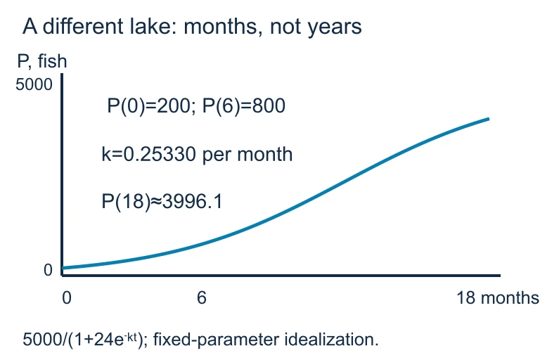For a lake with carrying capacity 5,000 fish and 200 fish initially, observing 800 fish at 6 months determines k ≈ 0.2533 per month. The model predicts about 3,996 fish at 18 months.

SECTION 7

Strengths and Limitations of DE Models

Differential equation models are among the most versatile tools in applied mathematics, but like all models, they make simplifying assumptions that limit their applicability. Understanding these trade-offs is important not only for the AP exam—where you may be asked to evaluate the appropriateness of a model—but also for scientific literacy more broadly. The table below summarizes the key strengths and limitations of the models covered in this lesson.

Aspect	Strengths	Limitations
Exponential Model	Simple, analytically solvable; excellent short-term approximation for many growth/decay processes; half-life and doubling time easily computed	Predicts infinite growth (unrealistic for bounded populations); no carrying capacity; fails for long-term biological or economic forecasting
Logistic Model	Incorporates a natural upper bound (carrying capacity); realistic S-curve behavior; inflection point analysis reveals peak growth	Assumes constant carrying capacity; does not account for seasonal variation, predator–prey interactions, or migration; symmetric about inflection
Newton's Cooling	Accurate for moderate temperature differences; widely applicable to thermodynamics, pharmacokinetics, and mixing problems	Assumes constant ambient temperature; breaks down for very large temperature gradients where radiation effects dominate; assumes uniform object temperature
General Separable DEs	Flexible; can model custom scenarios; separation of variables yields exact solutions when integrals are tractable	Not all DEs are separable; resulting integrals may not have closed-form antiderivatives; requires careful domain analysis

Strengths and limitations of the four model types studied in AP Calculus BC

✦

KEY TAKEAWAY

A differential equation model is like a flight simulator: it captures the essential dynamics—thrust, gravity, wind resistance—well enough to train pilots and predict behavior, but it deliberately omits minor details like the exact pattern of turbulence at every point. The exponential model is a simple glider simulation; the logistic model adds fuel capacity limits; Newton's cooling model adds thermal physics. More complex reality requires more complex models, but on the AP exam, these three "simulators" cover the vast majority of scenarios you will encounter.

SECTION 8

Connection to Advanced Differential Equations

The modeling techniques you learn in AP Calculus BC are the foundation for an entire branch of mathematics studied in college-level courses on ordinary and partial differential equations. The single-variable, first-order, separable equations on the BC exam are the simplest members of a much larger family. Understanding how these simple models connect to more advanced theory helps you appreciate both their power and their limitations.

AP Calculus BC Topic	Advanced Extension	What Changes
Exponential growth: dy/dt = ky	Systems of ODEs (e.g., predator–prey Lotka–Volterra)	Multiple interacting populations; two or more coupled DEs
Logistic: dy/dt = ky(1 − y/L)	Bifurcation theory; delayed logistic equations	Carrying capacity varies; time delays cause oscillations
Newton's cooling: dT/dt = k(T − Tₑ)	Heat equation (PDE): ∂T/∂t = α ∂²T/∂x²	Temperature varies in space as well as time; partial derivatives
Slope fields (qualitative analysis)	Phase plane analysis; stability theory	Classify equilibria as stable, unstable, or semi-stable using eigenvalues
Euler's method (numerical)	Runge–Kutta methods; adaptive step sizes	Higher-order accuracy; error control; computational efficiency

How AP Calculus BC models connect to college-level differential equations

If you pursue a STEM degree, you will almost certainly take a full course in differential equations, where you'll encounter linear systems, matrix methods, Laplace transforms, and Fourier series. The modeling instincts you develop now—translating rates into equations, recognizing equilibria, and interpreting solution behavior—will transfer directly. The AP Calculus BC exam tests these foundational instincts more than it tests computational complexity, so focus on building conceptual fluency with these core models.

SECTION 9

Practice Problems

Question 1: CONCEPTUAL

A chemical substance decomposes at a rate proportional to the amount present. If y(t) represents the amount of the substance at time t, which differential equation models this situation?

A. dy/dt = kt
B. dy/dt = −ky, where k > 0
C. dy/dt = ky², where k > 0
D. dy/dt = k/y, where k > 0
E. dy/dt = ky(1 − y), where k > 0

Show answer (B)

The correct answer is B. The phrase "rate proportional to the amount present" translates to dy/dt = ky, and "decomposes" indicates a decrease, so the proportionality constant must be negative—written as −k with k > 0. Choice A is incorrect because it makes the rate proportional to time rather than to y. Choice C is incorrect because it makes the rate proportional to y² rather than y. Choice D is incorrect because it makes the rate inversely proportional to y. Choice E is incorrect because it represents logistic growth, which would require the rate to be proportional to both y and (1 − y)—a condition not stated in the problem.

Question 2: BASIC CALCULATION

A population P(t) satisfies dP/dt = 0.03P with P(0) = 500. What is the population when t = 10?

A. 500e⁰·³ ≈ 675
B. 500(1.03)¹⁰ ≈ 672
C. 500 + 0.03(10) = 500.3
D. 500e³ ≈ 10,043
E. 500e⁻⁰·³ ≈ 370

Show answer (A)

The correct answer is A. The solution to dP/dt = 0.03P with P(0) = 500 is P(t) = 500e⁰·⁰³ᵗ. At t = 10, P(10) = 500e⁰·⁰³⁽¹⁰⁾ = 500e⁰·³ ≈ 500(1.3499) ≈ 675. Choice B confuses continuous exponential growth (eᵏᵗ) with discrete compounding ((1 + k)ᵗ)—these are different models. Choice C treats the differential equation as if dy/dt = 0.03 (a constant rate), ignoring the proportionality to P. Choice D incorrectly computes the exponent as 0.03 × 10 = 3 instead of 0.3. Choice E uses a negative exponent, which would model decay rather than growth.

Question 3: INTERMEDIATE

A population of bacteria grows logistically according to dP/dt = 0.5P(1 − P/1000). At what population level is the rate of growth the greatest?

A. P = 0
B. P = 250
C. P = 500
D. P = 750
E. P = 1000

Show answer (C)

The correct answer is C. For a logistic equation dP/dt = kP(1 − P/L), the right-hand side is a quadratic in P: 0.5P − 0.5P²/1000. This quadratic is maximized at P = L/2 = 1000/2 = 500, which can be verified by taking the derivative of dP/dt with respect to P and setting it to zero, or by recognizing that a downward-opening parabola achieves its vertex at the midpoint of its roots (P = 0 and P = 1000). Choice A is wrong because at P = 0 the growth rate is zero. Choice B (P = 250) has no special significance in this equation. Choice D (P = 750) gives a growth rate of 0.5(750)(0.25) = 93.75, which is less than the maximum at P = 500 where the rate is 0.5(500)(0.5) = 125. Choice E is wrong because at P = 1000 the growth rate is zero (the population is at carrying capacity).

Question 4: APPLIED

5 pts

A cup of coffee is initially at 95°C and is placed in a room where the ambient temperature is 22°C. After 5 minutes, the coffee has cooled to 80°C. (a) Write a differential equation that models the temperature T(t) of the coffee at time t minutes. (b) Solve the differential equation using the given information to find T(t). (c) Find the temperature of the coffee after 15 minutes. (d) At what time does the coffee reach 40°C?

Show answer

Rubric (5 points): (a) [1 point] The rate of temperature change is proportional to the difference between the coffee's temperature and the ambient temperature. The differential equation is dT/dt = k(T − 22), where k < 0 (since the coffee is cooling). Award 1 point for a correct DE with the correct ambient temperature. (b) [2 points — 1 for general solution, 1 for finding k] The general solution is T(t) = 22 + (95 − 22)eᵏᵗ = 22 + 73eᵏᵗ. Using T(5) = 80: 80 = 22 + 73e⁵ᵏ → 58 = 73e⁵ᵏ → e⁵ᵏ = 58/73 → 5k = ln(58/73) ≈ −0.22957 → k ≈ −0.04591. The particular solution is T(t) = 22 + 73e⁻⁰·⁰⁴⁵⁹¹ᵗ. Award 1 point for the correct general solution with initial condition applied, and 1 point for correctly finding k. (c) [1 point] T(15) = 22 + 73e⁻⁰·⁰⁴⁵⁹¹⁽¹⁵⁾ = 22 + 73e⁻⁰·⁶⁸⁸⁷ = 22 + 73(0.5024) ≈ 22 + 36.67 ≈ 58.7°C. Award 1 point for a correct numerical answer (accept 58–59°C with supporting work). (d) [1 point] Set T(t) = 40: 40 = 22 + 73e⁻⁰·⁰⁴⁵⁹¹ᵗ → 18 = 73e⁻⁰·⁰⁴⁵⁹¹ᵗ → e⁻⁰·⁰⁴⁵⁹¹ᵗ = 18/73 → −0.04591t = ln(18/73) ≈ −1.399 → t ≈ 30.5 minutes. Award 1 point for a correct answer with valid algebra.

Question 5: CRITICAL THINKING

3 pts

A student claims that the differential equation dy/dt = 0.1y(1 − y/500) with y(0) = 600 has no logistic solution because the initial value exceeds the carrying capacity. Evaluate this claim. Describe the qualitative behavior of y(t) for t > 0, including whether y(t) is increasing or decreasing, and identify any equilibria and their stability.

Show answer

Rubric (3 points): [1 point] The student's claim is incorrect. The logistic differential equation is valid for initial conditions above the carrying capacity. The formula P(t) = L / (1 + Ae⁻ᵏᵗ) still applies; with y(0) = 600 and L = 500, we get A = (500 − 600)/600 = −1/6. The value A < 0 is mathematically permissible and yields a solution that approaches L from above. [1 point] When y = 600 > L = 500, the factor (1 − y/500) = (1 − 600/500) = −0.2 is negative. Since 0.1y is positive and (1 − y/500) is negative, dy/dt < 0, meaning y(t) is decreasing. The population declines toward the carrying capacity because resources are insufficient to sustain 600 individuals. [1 point] The equilibria occur where dy/dt = 0: at y = 0 (unstable, since small positive populations grow) and y = 500 (stable, since populations above 500 decrease and populations below 500 increase). As t → ∞, y(t) → 500. The solution curve approaches L = 500 from above, which is the mirror image of the typical S-curve that approaches from below.

SUMMARY

Lesson Summary

Summary

Modeling with differential equations is the art of translating verbal descriptions of rates of change into precise mathematical equations. The three fundamental models on the AP Calculus BC exam are exponential growth/decay (dy/dt = ky), logistic growth (dy/dt = ky(1 − y/L)), and Newton's Law of Cooling (dT/dt = k(T − Tₑ)). Each arises from a specific verbal pattern involving the word "proportional" and can be identified by recognizing whether the rate depends on y alone, on y and a limiting factor, or on the difference between y and a constant.

Key skills include writing the DE from a word problem, applying an initial condition to find the particular solution, identifying equilibrium solutions (where dy/dt = 0), classifying their stability, and recognizing characteristic curve shapes (J-curve, S-curve, asymptotic decay). For the logistic model, remember that the maximum growth rate occurs at y = L/2, which corresponds to the inflection point of the solution curve. Mastery of these models provides the foundation for both the AP exam and future study in differential equations.