Logistic Models with Differential Equations - AP Calculus BC

SECTION 1

Historical Context & Motivation

In the late eighteenth century, Thomas Malthus warned that unchecked human population would grow exponentially, outstripping food supply and leading to catastrophe. His model, dP/dt = kP, predicted unbounded growth — a mathematical conclusion that troubled both economists and natural philosophers. While exponential models captured the early phase of population expansion, they failed spectacularly over longer time horizons because no real population grows without constraint. Resources deplete, disease spreads, and competition intensifies as a population nears the capacity of its environment.

The need for a more realistic model drove the Belgian mathematician Pierre-François Verhulst to introduce a self-limiting growth term in 1838. His logistic equation incorporated a carrying capacity — the maximum population an environment can sustain indefinitely. The logistic model predicts rapid initial growth that gradually decelerates as the population approaches this ceiling, producing the characteristic S-shaped (sigmoid) curve. This elegant modification resolved the paradox of infinite growth and became one of the most widely applied differential equations in biology, ecology, epidemiology, and even marketing.

1798 • Malthus Publishes Exponential Growth Model

Thomas Malthus argues in An Essay on the Principle of Population that populations grow geometrically while resources grow arithmetically, predicting inevitable famine.

1838 • Verhulst Proposes the Logistic Equation

Pierre-François Verhulst modifies the exponential model by introducing a carrying capacity L, publishing the logistic differential equation dP/dt = kP(1 − P/L) in Correspondance Mathématique et Physique.

1920 • Pearl & Reed Rediscover the Logistic Curve

Raymond Pearl and Lowell Reed independently rediscover the logistic function while modeling U.S. census data, demonstrating its predictive power for human population trends.

1927 • Kermack–McKendrick Epidemic Model

The logistic framework is adapted to model the spread of infectious disease, laying the foundation for the SIR compartmental model used throughout modern epidemiology.

Present • Logistic Models on the AP Calculus BC Exam

The College Board includes logistic differential equations as a required topic in AP Calculus BC, testing students' ability to set up, solve, and interpret these models in context.

The central question the logistic model addresses is: How does a quantity grow when its rate of increase depends not only on its current size but also on how close it is to a maximum capacity? This question lies at the heart of many AP Calculus BC free-response and multiple-choice problems involving differential equations.

SECTION 2

Core Principles & Definitions

Before diving into the mathematics, it is essential to understand the conceptual building blocks that distinguish the logistic model from simpler growth models. The logistic differential equation rests on a few fundamental ideas, each of which carries specific mathematical meaning that you will encounter repeatedly on the AP exam.

Carrying Capacity (L)

The carrying capacity L (sometimes written as M or K) is the maximum value the population or quantity can attain. It is a horizontal asymptote of the solution curve: as t → ∞, P(t) → L.

Intrinsic Growth Rate (k)

The constant k represents the growth rate when the population is small relative to L. In this regime the factor (1 − P/L) ≈ 1, so dP/dt ≈ kP, recovering the exponential model.

Self-Limiting Factor (1 − P/L)

The factor (1 − P/L) acts as a brake. When P is near 0, this factor is near 1 and growth is fast. When P approaches L, this factor approaches 0 and growth stalls. If P ever exceeds L, the factor becomes negative and the population decreases.

Inflection Point at P = L/2

The solution curve has an inflection point when P = L/2. At this value the growth rate dP/dt is maximized, and the curve transitions from concave up to concave down. This is a high-frequency AP exam topic.

Equilibrium Solutions

Setting dP/dt = 0 yields two equilibrium solutions: P = 0 (unstable) and P = L (stable). Any solution starting between 0 and L will increase toward L; a solution starting above L will decrease toward L.

✦

KEY TAKEAWAY

Think of logistic growth like filling a concert venue. When the venue is nearly empty, people stream in quickly through all entrances. As the venue fills, congestion builds at the doors and the flow slows dramatically. Eventually, when the venue reaches capacity, the net inflow effectively stops. The carrying capacity L is the venue's maximum occupancy, and the factor (1 − P/L) quantifies how much room remains. The fastest rate of entry — the moment the crowd is pouring in most rapidly — occurs when the venue is exactly half full, which corresponds to the inflection point P = L/2.

SECTION 3

Visual Explanation — The Logistic Curve

The signature shape of the logistic model is the S-curve (sigmoid curve). The diagram below plots a logistic solution P(t) against time, illustrating the three distinct phases of growth: the early exponential phase, the inflection transition, and the asymptotic approach to carrying capacity. Pay close attention to the location of the inflection point and the dashed carrying-capacity line — these features are tested heavily on the AP exam.

The logistic solution curve passes through three phases. Phase I (cyan) shows near-exponential growth when P is small. At the inflection point (violet dot, P = L/2), growth rate dP/dt is maximized. In Phase III (pink), the curve levels off as P → L (amber dashed line).

Notice how the concavity of the curve changes at the inflection point t*. For t < t*, the curve is concave up (the population is accelerating). For t > t*, the curve is concave down (the population is still growing but decelerating). This concavity change is directly tied to the second derivative d²P/dt², which the AP exam frequently asks you to analyze.

SECTION 4

Mathematical Framework

The mathematical heart of the logistic model is a first-order, separable, nonlinear differential equation. In this section we present the standard form of the equation, derive its general solution via partial fractions, and establish the key formulas you need for the AP exam.

THE LOGISTIC DIFFERENTIAL EQUATION

dP/dt = kP(1 − P/L)

P = P(t) is the population at time t; k > 0 is the intrinsic growth rate; L > 0 is the carrying capacity. The product of the two factors kP and (1 − P/L) ensures growth is fastest at intermediate values and vanishes at P = 0 and P = L.

Solving by Separation of Variables

The logistic DE is separable. Rewriting dP/dt = kP(1 − P/L) and separating variables yields:

SEPARATION STEP

∫ dP / [P(1 − P/L)] = ∫ k dt

The left side is integrated using partial fraction decomposition: 1/[P(1 − P/L)] = 1/P + (1/L)/(1 − P/L). After integrating both sides and solving for P, we obtain the general solution.

GENERAL SOLUTION

P(t) = L / (1 + Ae⁻ᵏᵗ) where A = (L − P₀)/P₀

P₀ = P(0) is the initial population. The constant A is determined by the initial condition. As t → ∞, e⁻ᵏᵗ → 0 so P(t) → L. When P₀ < L, A > 0 and the solution increases toward L. When P₀ > L, A < 0 and the solution decreases toward L.

MAXIMUM GROWTH RATE

(dP/dt)_max = kL/4 occurring when P = L/2

Substituting P = L/2 into the DE: dP/dt = k(L/2)(1 − 1/2) = kL/4. This result is critical: the AP exam frequently asks for the population value at which the rate of change is greatest.

⚠

AP Exam Tip

The logistic DE often appears in the form dP/dt = kP(1 − P/L), but it may also be written as dP/dt = (k/L) × P(L − P). These are algebraically identical. Always check which form the problem uses before identifying k and L. A common trap is misidentifying k when the equation is given in the second form — the coefficient of the product P(L − P) is k/L, not k.

SECTION 5

Slope Fields & Phase Line Analysis

On the AP exam you may be asked to sketch or interpret a slope field for the logistic DE or to perform a qualitative phase line analysis without solving the equation explicitly. Because the logistic DE is autonomous — the right-hand side depends only on P, not on t — the slope field has a special property: all line segments in a given horizontal strip (constant P) have the same slope. The phase line summarizes the behavior of dP/dt as a function of P alone, allowing you to determine stability of equilibria and the direction of change at a glance.

Left: The parabola dP/dt = kP(1 − P/L) is positive for 0 < P < L, reaching its maximum at P = L/2. Right: The phase line shows upward arrows (increasing P) between the unstable equilibrium P = 0 and the stable equilibrium P = L. If P > L, the population decreases back to L.

The left panel makes it clear why the maximum rate of change occurs at P = L/2: the graph of dP/dt versus P is a downward-opening parabola with roots at P = 0 and P = L, and the vertex of a parabola with roots at 0 and L lies at the midpoint P = L/2. This is a powerful shortcut — you never need to compute a second derivative to find the inflection point of the logistic solution. Simply recognize that the inflection occurs when the growth rate is maximized, i.e., at P = L/2.

💡

Concavity from the Rate Curve

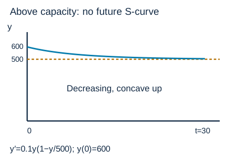When P < L/2, the rate curve is increasing (dP/dt rises as P grows), which means d²P/dt² > 0 and the solution is concave up. When P > L/2, the rate curve is decreasing, so d²P/dt² < 0 and the solution is concave down. This provides a quick qualitative sketch tool for AP free-response questions.

A population curve starts at 600 above the dashed carrying-capacity line 500 and decreases toward it from above, flattening as time advances. For y′ = 0.1 y(1 − y/500) with y(0) = 600, the initial rate is −12. The solution decreases toward 500 and is concave up for all future time; this trajectory has no future inflection point.Open full diagram

SECTION 6

Worked Example

Let us work through a complete AP-style problem. Suppose a fish population in a lake is modeled by the logistic differential equation:

GIVEN DIFFERENTIAL EQUATION

dP/dt = 0.5P(1 − P/8000)

where P is measured in fish and t in years. The initial population is P(0) = 1000.

Full Logistic Model Analysis

1
Step 1 — Identify Parameters

Comparing dP/dt = 0.5P(1 − P/8000) with the standard form dP/dt = kP(1 − P/L), we identify k = 0.5 per year and L = 8000 fish. The initial condition is P₀ = 1000.

k = 0.5, L = 8000, P₀ = 1000
2
Step 2 — Write the General Solution

The general solution is P(t) = L / (1 + Ae⁻ᵏᵗ). We compute A = (L − P₀)/P₀ = (8000 − 1000)/1000 = 7. Therefore:

P(t) = 8000 / (1 + 7e⁻⁰·⁵ᵗ)
3
Step 3 — Find the Population at t = 4 Years

Substitute t = 4: P(4) = 8000 / (1 + 7e⁻²). We compute e⁻² ≈ 0.1353, so 7e⁻² ≈ 0.9474. Then P(4) = 8000 / (1 + 0.9474) = 8000 / 1.9474 ≈ 4108 fish.

P(4) ≈ 4108 fish
4
Step 4 — Determine When Growth Rate Is Maximum

The growth rate dP/dt is maximized when P = L/2 = 4000. We solve 4000 = 8000/(1 + 7e⁻⁰·⁵ᵗ), giving 1 + 7e⁻⁰·⁵ᵗ = 2, so 7e⁻⁰·⁵ᵗ = 1, hence e⁻⁰·⁵ᵗ = 1/7. Taking the natural log: −0.5t = ln(1/7) = −ln 7, so t = 2 ln 7 ≈ 2(1.9459) ≈ 3.892 years.

Maximum growth rate occurs at t ≈ 3.892 years when P = 4000
5
Step 5 — Compute the Maximum Growth Rate

The maximum value of dP/dt equals kL/4 = (0.5)(8000)/4 = 1000 fish per year. Alternatively, substitute P = 4000 into the DE: dP/dt = 0.5(4000)(1 − 4000/8000) = 0.5(4000)(0.5) = 1000.

(dP/dt)_max = 1000 fish/year
6
Step 6 — Long-Term Behavior

As t → ∞, e⁻⁰·⁵ᵗ → 0, so P(t) → 8000/(1 + 0) = 8000. The population approaches the carrying capacity of 8000 fish but never exceeds it, confirming L = 8000 is a stable equilibrium.

lim(t→∞) P(t) = 8000 fish = L

Caretaker, aerator, habitat shelf, vegetation and fish establish a managed pond. Visible fish are illustrative individuals, not the model initial population or carrying capacity. Separate exact panel: Separate computed plots show a population trajectory from1000 toward8000 and a growth-rate parabola peaking at4000 with1000fish per year. For P′ = 0.5P(1 − P/8,000) with P(0) = 1,000, the population approaches 8,000 fish. Growth is fastest at 4,000 fish, about 3.89 years after the start.

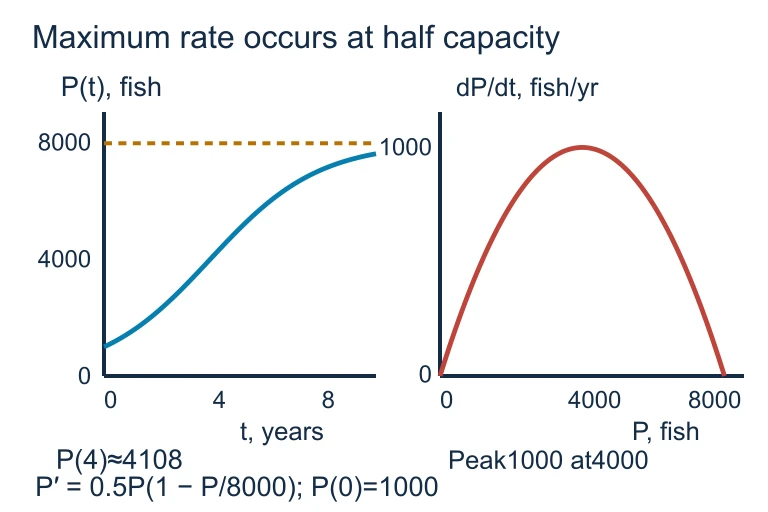For P′ = 0.5P(1 − P/8,000) with P(0) = 1,000, the population approaches 8,000 fish. Growth is fastest at 4,000 fish, about 3.89 years after the start.

SECTION 7

Comparing Exponential & Logistic Models

Understanding when and why to choose a logistic model over an exponential model is a critical skill on the AP exam. The table below contrasts the two models across all the features that commonly appear in exam questions.

Feature	Exponential Model	Logistic Model
Differential Equation	dP/dt = kP	dP/dt = kP(1 − P/L)
Solution	P(t) = P₀eᵏᵗ	P(t) = L / (1 + Ae⁻ᵏᵗ)
Long-Term Behavior	P → ∞ (unbounded growth)	P → L (bounded by carrying capacity)
Concavity	Always concave up (k > 0)	Concave up for P < L/2; concave down for P > L/2
Inflection Point	Does not exist	At P = L/2
Equilibria	P = 0 only (unstable)	P = 0 (unstable) and P = L (stable)
When to Use	Short-term, unlimited resources	Long-term, limited resources / saturation

Exponential vs. Logistic Growth Model Comparison

✦

KEY TAKEAWAY

The exponential model is the logistic model's special case when the population is negligibly small compared to the carrying capacity. Just as Newtonian mechanics is a limiting case of relativity at low speeds, exponential growth is the limiting case of logistic growth when P/L ≈ 0. Whenever a problem states that growth is limited, bounded, or approaching a maximum, the logistic model is the appropriate choice.

SECTION 8

Connection to Advanced Theory

The logistic differential equation is the gateway to a rich family of models studied in higher mathematics and applied science. While the AP Calculus BC exam focuses exclusively on the autonomous logistic DE and its closed-form solution, understanding where the model sits in the broader landscape helps you appreciate its elegance and its limitations.

AP Calculus BC (Logistic)	Advanced Extension
Single population: dP/dt = kP(1 − P/L)	Lotka–Volterra (predator–prey): system of coupled DEs for interacting species
Constant carrying capacity L	Time-varying capacity L(t) to model seasonal or changing environments
Deterministic closed-form solution	Stochastic logistic models with random noise (SDEs)
Continuous growth	Discrete logistic map: xₙ₊₁ = rxₙ(1 − xₙ), which can exhibit chaos
Separation of variables (exact solution)	Euler's method and Runge–Kutta for numerical approximation of non-separable DEs

AP Logistic Model vs. Advanced Extensions

One particularly striking extension is the discrete logistic map, x_n+1 = rx_n(1 − x_n), which Robert May studied in 1976. For small values of the parameter r, the discrete version converges to a stable equilibrium just like the continuous case. However, as r increases, the system undergoes period-doubling bifurcations and eventually exhibits deterministic chaos — an entirely unpredictable behavior arising from a deceptively simple equation. This connection between the smooth, predictable continuous logistic model and the chaotic discrete version illustrates the depth hidden in what initially appears to be a straightforward differential equation.

ℹ

Looking Ahead

If you continue to multivariable calculus or differential equations courses, you will encounter systems of DEs (like Lotka–Volterra) and numerical methods (like Euler's method, which is also on the AP Calculus BC exam). The logistic model provides excellent intuition for stability analysis, phase portraits, and qualitative reasoning — skills that transfer directly to those more advanced topics.

SECTION 9

Practice Problems

Question 1: CONCEPTUAL

A population P(t) is modeled by the logistic differential equation dP/dt = 0.3P(1 − P/5000). Which of the following statements is true about the solution P(t) when P(0) = 2500?

A. P(t) is increasing and concave up for all t > 0.
B. P(t) is increasing and concave down for all t > 0.
C. P(t) is decreasing and concave up for all t > 0.
D. P(t) is increasing with an inflection point at P = 2500.
E. P(t) approaches 0 as t → ∞.

Show answer (B)

Answer: B. Since P(0) = 2500 = L/2 = 5000/2, the population begins exactly at the inflection point. For P > L/2, the solution is concave down (d²P/dt² < 0) because the growth rate dP/dt is decreasing as P increases beyond L/2. Meanwhile, dP/dt = 0.3(2500)(1 − 0.5) = 375 > 0, so P is still increasing. Thus P(t) is increasing and concave down for all t > 0. A is wrong because concavity changes at P = L/2, and since P₀ = L/2, the curve is concave down (not up) for t > 0. C is wrong because P is increasing (dP/dt > 0 for 0 < P < L). D is wrong because although P = 2500 is the inflection point, the solution starts there and immediately moves into the concave-down region — it does not pass through the inflection for t > 0. E is wrong because P → L = 5000 as t → ∞, not 0.

Question 2: BASIC CALCULATION

A population satisfies dP/dt = 0.4P(1 − P/2000) with P(0) = 200. What is the value of P(t) as t → ∞?

A. 200
B. 1000
C. 2000
D. ∞
E. 500

Show answer (C)

Answer: C. The carrying capacity is L = 2000. For any logistic model with 0 < P₀ < L, the population approaches L as t → ∞. The solution is P(t) = 2000/(1 + 9e⁻⁰·⁴ᵗ) where A = (2000 − 200)/200 = 9. As t → ∞, e⁻⁰·⁴ᵗ → 0, yielding P → 2000. A is wrong — that is only the initial value. B is wrong — L/2 = 1000 is the inflection point, not the limiting value. D is wrong — unbounded growth occurs in the exponential model, not the logistic. E is wrong — 500 has no special significance in this model.

Question 3: INTERMEDIATE

The number of people who have heard a rumor in a school of 600 students is modeled by dN/dt = 0.002N(600 − N), where N(0) = 10. Find the maximum rate at which the rumor spreads and determine the explicit solution N(t).

A. Max rate = 180 people/day; N(t) = 600/(1 + 59e⁻¹·²ᵗ)
B. Max rate = 300 people/day; N(t) = 600/(1 + 59e⁻⁰·⁰⁰²ᵗ)
C. Max rate = 180 people/day; N(t) = 600/(1 + 590e⁻¹·²ᵗ)
D. Max rate = 90 people/day; N(t) = 600/(1 + 59e⁻⁰·⁶ᵗ)
E. Max rate = 180 people/day; N(t) = 300/(1 + 29e⁻¹·²ᵗ)

Show answer (A)

Answer: A. First, rewrite in standard form: dN/dt = 0.002N(600 − N) = (0.002 × 600)N(1 − N/600) = 1.2N(1 − N/600). So k = 1.2 and L = 600. The maximum rate is kL/4 = 1.2 × 600/4 = 180 people/day, occurring at N = 300. The constant A = (600 − 10)/10 = 59. The solution is N(t) = 600/(1 + 59e⁻¹·²ᵗ). B is wrong because it uses k = 0.002 in the exponential rather than k = 1.2; the coefficient 0.002 is k/L, not k. C is wrong because A = (600 − 10)/10 = 59, not 590. D is wrong because it uses k = 0.6 and max rate = kL/4 = 90, both arising from an incorrect identification of k. E is wrong because the carrying capacity is 600, not 300.

Question 4: APPLIED

5 pts

A biologist observes that a deer population in a national park satisfies dP/dt = 0.1P(1 − P/4000) with P(0) = 500. (a) Write the explicit solution P(t). (b) Find the time at which the population reaches 2000. (c) At what time is the population growing most rapidly? What is that rate? (d) Interpret the meaning of lim(t→∞) P(t) in the context of this problem.

Show answer

Rubric (5 points): Point 1 — (a) Explicit solution: Identify k = 0.1, L = 4000. Compute A = (4000 − 500)/500 = 7. Solution: P(t) = 4000/(1 + 7e⁻⁰·¹ᵗ). Point 2 — (b) Time to reach P = 2000: Set 2000 = 4000/(1 + 7e⁻⁰·¹ᵗ). Solve: 1 + 7e⁻⁰·¹ᵗ = 2, so 7e⁻⁰·¹ᵗ = 1, e⁻⁰·¹ᵗ = 1/7, −0.1t = −ln 7, t = 10 ln 7 ≈ 19.459 years. Point 3 — (c) Maximum growth rate and timing: The growth rate is maximized at P = L/2 = 2000, which occurs at t = 10 ln 7 ≈ 19.459 years (same as part (b)). The maximum rate is kL/4 = (0.1)(4000)/4 = 100 deer per year. Point 4 — (d) Interpretation of limit: lim(t→∞) P(t) = 4000. In context, the deer population will approach but never exceed 4000 deer, which represents the maximum number of deer the park's resources can sustain indefinitely. Point 5 — Communication & notation: Proper use of units (deer, years), correct notation for limits, and clear connection between mathematical results and the biological context.

Question 5: CRITICAL THINKING

4 pts

Consider the differential equation dP/dt = kP(1 − P/L). (a) Show that d²P/dt² = k²P(1 − P/L)(1 − 2P/L). (b) Use this result to prove rigorously that the inflection point of P(t) occurs at P = L/2. (c) Explain why, for any initial value 0 < P₀ < L/2, the solution P(t) must have exactly one inflection point.

Show answer

Rubric (4 points): Point 1 — (a) Deriving d²P/dt²: Differentiate dP/dt = kP − kP²/L with respect to t using the chain rule: d²P/dt² = (k − 2kP/L)(dP/dt) = (k − 2kP/L) × kP(1 − P/L) = k²P(1 − P/L)(1 − 2P/L). Point 2 — (b) Proving inflection at P = L/2: An inflection point occurs where d²P/dt² = 0 and changes sign. The factors of d²P/dt² are k²P, (1 − P/L), and (1 − 2P/L). For 0 < P < L, the first two factors are positive, so d²P/dt² = 0 only when 1 − 2P/L = 0, i.e., P = L/2. Since (1 − 2P/L) changes sign from positive (P < L/2) to negative (P > L/2), this is indeed an inflection point. Point 3 — (c) Exactly one inflection point: When P₀ < L/2, the solution P(t) is strictly increasing with P(t) → L. Since P is continuous and increases from P₀ < L/2 to L > L/2, by the Intermediate Value Theorem P must pass through L/2 exactly once. Before reaching L/2, d²P/dt² > 0 (concave up); after passing L/2, d²P/dt² < 0 (concave down). Since P is monotonically increasing, it crosses L/2 exactly once, yielding exactly one inflection point. Point 4 — Justification quality: Full credit requires clear chain rule computation, correct sign analysis of all three factors, and explicit invocation of the Intermediate Value Theorem or equivalent rigorous argument for uniqueness.

SUMMARY

Lesson Summary

Summary

The logistic differential equation dP/dt = kP(1 − P/L) models growth that is self-limiting due to a finite carrying capacity L. Its general solution, P(t) = L/(1 + Ae⁻ᵏᵗ) where A = (L − P₀)/P₀, produces the signature S-shaped sigmoid curve. The solution has two equilibrium solutions: P = 0 (unstable) and P = L (stable). A central result is that the maximum growth rate is kL/4 and occurs at the inflection point P = L/2, where the solution transitions from concave up to concave down.

For the AP exam, remember these essential skills: (1) identify k and L from any algebraic form of the DE, (2) write the explicit solution using the initial condition, (3) compute the long-term limit (always L for 0 < P₀ < ∞), (4) find the inflection point and maximum rate, and (5) interpret results in context with proper units. The logistic model stands in contrast to unbounded exponential growth, and its qualitative features — slope fields, phase lines, and concavity analysis — are among the most frequently tested topics on the differential equations portion of the AP Calculus BC exam.