Introduction to Optimization Problems - AP Calculus BC

SECTION 1

Historical Context & Motivation

The desire to find the "best" outcome—the greatest area, the shortest distance, the least cost—predates calculus itself, reaching back to antiquity when geometers sought the shapes that enclosed the most space. Optimization, the mathematical discipline of finding maximum or minimum values of a function subject to given constraints, crystallized only after Newton and Leibniz provided the tools of differential calculus. Once the derivative was understood as a measure of instantaneous rate of change, mathematicians could rigorously identify the exact points at which a quantity peaks or bottoms out, transforming intuitive guesses into provable conclusions. This section traces the key milestones that brought optimization from geometric curiosity to a cornerstone of applied mathematics.

~300 BCE • The Isoperimetric Problem

Greek geometers, including Zenodorus, investigated which closed curve of a given perimeter encloses the greatest area—a circle. This is arguably the earliest recorded optimization problem, solved without calculus by symmetry arguments.

1638 • Fermat's Method of Adequality

Pierre de Fermat developed a proto-derivative technique called adequality, equating a function's value at x and at x + ε and then letting ε vanish. He used it to find tangent lines and, crucially, to locate maxima and minima of polynomial expressions.

1684–1687 • Newton & Leibniz Formalize Calculus

The independent invention of calculus by Isaac Newton and Gottfried Wilhelm Leibniz gave a general, systematic way to compute derivatives and thereby solve optimization problems on arbitrary differentiable functions.

1744 • Euler and the Calculus of Variations

Leonhard Euler extended optimization from finite-dimensional problems to functionals—finding entire curves that minimize quantities like arc length or potential energy. This laid the groundwork for modern physics and engineering optimization.

1947–present • Linear & Nonlinear Programming

George Dantzig's simplex method and subsequent advances in nonlinear programming brought optimization into industry, economics, and computer science, building directly on the calculus-based ideas of finding critical points.

The central question optimization addresses is deceptively simple: given a real-valued function f defined on some domain, at which input x does f achieve its greatest (or smallest) value? In AP Calculus BC, you will encounter this question in two primary forms—finding absolute extrema on a closed interval, and constructing and optimizing a function that models a real-world scenario with constraints. Both forms rely on a single powerful idea: if f is differentiable at a point where an extremum occurs in the interior of its domain, then f ′ must equal zero there. Understanding how to wield this fact—together with the Extreme Value Theorem, the First and Second Derivative Tests, and careful domain analysis—is the gateway to solving optimization problems with confidence.

SECTION 2

Core Principles & Definitions

Before diving into worked examples, it is essential to internalize the foundational ideas that underpin every optimization problem. These principles are not merely procedural steps; they form the logical skeleton that justifies why the methods work. The four core concepts below—critical points, the Extreme Value Theorem, the Closed-Interval Method, and constrained optimization—appear in virtually every AP Calculus optimization question.

Critical Points

A critical point of f is a value c in the domain of f where f ′(c) = 0 or f ′(c) does not exist. Every local extremum of f on an open interval must occur at a critical point (Fermat's Theorem), making these points the natural candidates to check.

Extreme Value Theorem (EVT)

If f is continuous on a closed interval [a, b], then f attains both an absolute maximum and an absolute minimum on [a, b]. This theorem guarantees existence, ensuring that our search for extreme values will always succeed when the hypotheses are met.

Closed-Interval Method

To find absolute extrema of a continuous function on [a, b]: (1) find all critical points in (a, b), (2) evaluate f at each critical point and at the endpoints a and b, (3) the largest value is the absolute maximum, the smallest is the absolute minimum.

Constrained Optimization

In applied problems, the quantity to optimize (the objective function) depends on multiple variables linked by a constraint equation. Use the constraint to eliminate all but one variable, then apply single-variable calculus to find the optimum.

✦

KEY TAKEAWAY

Think of an optimization problem like tuning a radio dial. The objective function is the signal strength, the constraint is the range of frequencies your radio can receive, and the critical points are the positions where the signal peaks or dips. You slide the dial across the full range (endpoints included) and note every peak and valley; the loudest signal among them is your absolute maximum. Calculus gives you the exact "dial positions" to check by setting the derivative to zero.

SECTION 3

Visual Explanation — Anatomy of an Optimization Problem

The diagram below illustrates the Closed-Interval Method applied to a continuous function on [a, b]. Notice how the absolute maximum does not necessarily occur at a critical point where f ′ = 0; it can also occur at an endpoint. Similarly, the absolute minimum may reside at either a critical point or an endpoint. The candidates for absolute extrema are highlighted, and vertical dashed lines mark the critical points where f ′(c) = 0.

The curve represents a continuous function on [a, b]. Cyan dots mark the endpoints; amber dots mark critical points where f ′ = 0; the pink dot at c₃ is the absolute maximum. The absolute minimum occurs at the left endpoint a. The Closed-Interval Method compares f-values at all marked points to identify the global extrema.

This visualization encapsulates the entire strategy: once you locate every critical point within (a, b) and evaluate f at each one alongside the two endpoints, the problem reduces to a simple comparison of finitely many real numbers. The elegance of the Closed-Interval Method is that it sidesteps the need for the First or Second Derivative Test entirely when the domain is a closed interval—every candidate is on equal footing, and the largest and smallest values reveal themselves immediately.

SECTION 4

Mathematical Framework

The mathematical backbone of optimization rests on a small number of powerful theorems and derivative tests. In this section, we formalize the conditions that guarantee the existence of extrema and present the primary tests used to classify critical points. These tools apply not only to textbook functions but also to the applied modeling problems that dominate the AP Calculus BC exam.

FERMAT'S THEOREM (NECESSARY CONDITION)

If f has a local extremum at c and f ′(c) exists, then f ′(c) = 0.

This theorem provides only a necessary condition, not a sufficient one. The converse is false: f ′(c) = 0 does not guarantee an extremum (consider f(x) = x³ at x = 0).

FIRST DERIVATIVE TEST

If f ′ changes from + to − at c, then f(c) is a local maximum. If f ′ changes from − to + at c, then f(c) is a local minimum.

Check the sign of f ′ on both sides of each critical point. A sign change confirms an extremum; no sign change means the critical point is neither a max nor a min (e.g., an inflection point with a horizontal tangent).

SECOND DERIVATIVE TEST

If f ′(c) = 0 and f ″(c) > 0, then f(c) is a local minimum. If f ′(c) = 0 and f ″(c) < 0, then f(c) is a local maximum.

When f ″(c) = 0, the test is inconclusive. In that case, revert to the First Derivative Test or higher-order derivative analysis. The Second Derivative Test is especially efficient for problems where computing f ″ is straightforward.

GENERAL OPTIMIZATION PROCEDURE (APPLIED PROBLEMS)

1. Identify the objective function Q to maximize or minimize. 2. Express Q in terms of a single variable using the constraint equation. 3. Determine the feasible domain for that variable. 4. Find critical points and evaluate Q at critical points and endpoints.

The constraint equation typically arises from a geometric or physical relationship (e.g., a fixed perimeter, a fixed volume of material, or a budget). Eliminating a variable converts the multivariable problem into a single-variable calculus problem.

💡

AP Exam Tip

On the AP Calculus BC exam, justification is essential. If a free-response question asks you to find an absolute maximum, you must explain why your answer is absolute—either by citing the Extreme Value Theorem and comparing all candidates, or by demonstrating that the critical point is the only one in the domain and using a sign analysis or the Second Derivative Test.

SECTION 5

Detailed Breakdown — Common Optimization Problem Types

Optimization problems on the AP Calculus BC exam fall into recognizable categories. While the surface details change—boxes, fences, distances, revenues—the underlying structure is remarkably consistent. The diagram below maps out the decision process you should follow, and the table that follows classifies the most common problem archetypes along with their typical objective functions and constraints.

Follow this six-step flowchart for every applied optimization problem. Each colored box corresponds to a distinct phase: identifying the objective (cyan), identifying the constraint (pink), reducing to one variable (amber), determining the domain (emerald), finding critical points (orange), and justifying the answer (red).

Problem Type	Objective Function	Typical Constraint	Key Insight
Area Maximization	A = ℓ × w (rectangle), or A = πr² (circle sector), etc.	Fixed perimeter or fixed amount of fencing	Eliminate one dimension using the perimeter constraint; optimal shape is often a square.
Volume Optimization	V = x(L − 2x)(W − 2x) for an open-top box, V = πr²h for a cylinder	Fixed surface area or sheet dimensions	Express h in terms of r (or vice versa) using the surface-area formula.
Minimum Distance	D² = (x − a)² + (f(x) − b)² (often minimize D² to avoid the square root)	Point lies on a given curve y = f(x)	Minimizing D² gives the same critical points as minimizing D, but the algebra is simpler.
Cost / Revenue	C(x) = fixed + variable × x, or R(x) = p(x) × x	Demand function p = p(x), or budget constraint	Profit P = R − C; maximize P by setting P ′(x) = 0 (marginal revenue = marginal cost).

Common AP Calculus BC optimization problem archetypes

SECTION 6

Worked Example — Maximizing the Volume of an Open-Top Box

A manufacturer wants to create an open-top box by cutting equal squares of side length x from each corner of a rectangular sheet of cardboard that measures 24 cm by 16 cm, and then folding up the resulting flaps. What value of x maximizes the volume of the box?

Open-Top Box Optimization

1
Step 1 — Draw a diagram and define variables

After cutting squares of side length x from each corner, the base of the box has length 24 − 2x and width 16 − 2x. The height of the box equals x. Our objective function is the volume V.
2
Step 2 — Write the objective function

The volume of the box is V(x) = x(24 − 2x)(16 − 2x). Expanding: V(x) = x(384 − 48x − 32x + 4x²) = x(384 − 80x + 4x²) = 4x³ − 80x² + 384x.

V(x) = 4x³ − 80x² + 384x
3
Step 3 — Determine the feasible domain

Each dimension must be positive. We need x > 0, 24 − 2x > 0 (so x < 12), and 16 − 2x > 0 (so x < 8). The binding constraint is x < 8, giving the feasible domain 0 < x < 8. Since V(0) = 0 and V(8) = 0, we can treat this as the closed interval [0, 8] for the Extreme Value Theorem, though the endpoints yield degenerate boxes with zero volume.

Feasible domain: 0 ≤ x ≤ 8
4
Step 4 — Find critical points by setting V ′(x) = 0

Differentiate: V ′(x) = 12x² − 160x + 384. Factor out 4: V ′(x) = 4(3x² − 40x + 96). Set the quadratic to zero: 3x² − 40x + 96 = 0. By the quadratic formula, x = (40 ± √(1600 − 1152)) / 6 = (40 ± √448) / 6 = (40 ± 4√28) / 6 = (40 ± 8√7) / 6. Numerically, √7 ≈ 2.6458, so 8√7 ≈ 21.166. Thus x ≈ (40 − 21.166)/6 ≈ 3.139 or x ≈ (40 + 21.166)/6 ≈ 10.194. Since 10.194 > 8, it lies outside the feasible domain.

Only critical point in [0, 8]: x = (20 − 4√7)/3 ≈ 3.14 cm
5
Step 5 — Evaluate V at the critical point and endpoints

V(0) = 0 and V(8) = 0 (degenerate boxes). At x ≈ 3.139: V(3.139) = 3.139 × (24 − 6.278) × (16 − 6.278) = 3.139 × 17.722 × 9.722 ≈ 3.139 × 172.29 ≈ 540.9 cm³.

Maximum volume ≈ 540.9 cm³ at x = (20 − 4√7)/3 ≈ 3.14 cm
6
Step 6 — Justify the result

Since V is continuous on [0, 8] and the only critical point in the interior yields a value greater than V at both endpoints, the Extreme Value Theorem guarantees that this is the absolute maximum. Alternatively, one can verify via the Second Derivative Test: V ″(x) = 24x − 160, so V ″(3.139) ≈ 24(3.139) − 160 ≈ −84.66 < 0, confirming a local maximum. Since it is the only critical point in (0, 8), it must be the absolute maximum.

A cardboard net with four corner squares removed, partly folded walls, and a finished open-top box on a worktable. For a 24 cm × 16 cm sheet, V(x) = x(24 − 2x)(16 − 2x), with 0 < x < 8. The maximizing cut is x = (20 − 4√7)/3 cm, about 3.14 cm.

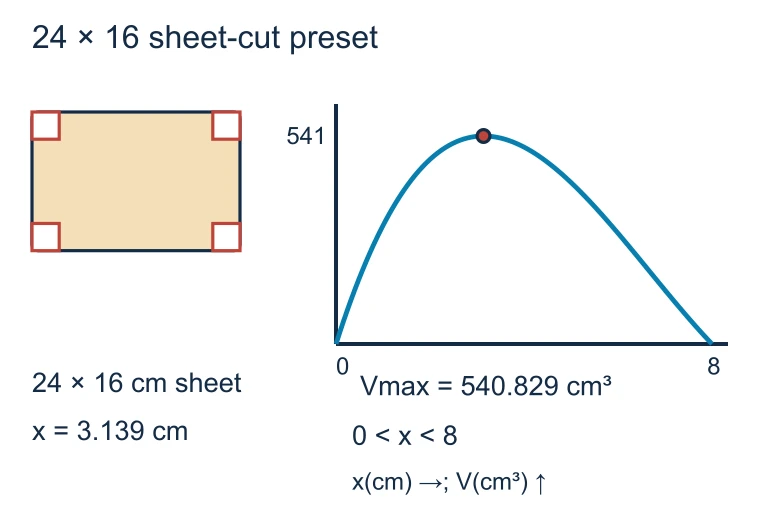For a 24 cm × 16 cm sheet, V(x) = x(24 − 2x)(16 − 2x), with 0 < x < 8. The maximizing cut is x = (20 − 4√7)/3 cm, about 3.14 cm.

SECTION 7

Comparing Justification Methods

On the AP exam, choosing the right justification method can save time and ensure full credit. The Closed-Interval Method, the First Derivative Test, and the Second Derivative Test each have distinct strengths and limitations. The table below compares them so that you can select the most efficient approach for each problem.

Method	When to Use	Strengths	Limitations
Closed-Interval Method	f is continuous on a closed interval [a, b]	Guaranteed by EVT; straightforward comparison of finitely many values; no sign analysis needed	Only works on closed intervals; requires evaluating f at every critical point and endpoint
First Derivative Test	Open or half-open domains; when f ″ is hard to compute	Works even when f ″ doesn't exist; identifies local extrema on open intervals	Requires sign analysis on both sides of the critical point; must separately argue that a local extremum is absolute
Second Derivative Test	f ′(c) = 0 and f ″(c) is easy to compute and nonzero	Quick—just evaluate f ″ at the critical point; gives concavity information	Inconclusive when f ″(c) = 0; requires f ″ to exist; only identifies local extrema—must still argue absolute

Comparison of justification methods for optimization problems

✦

KEY TAKEAWAY

In engineering design, one often encounters a feasible region defined by physical constraints (e.g., dimensions must be positive, materials are finite). When this region corresponds to a closed interval—or when the objective function blows up or approaches zero at the boundary of an open domain—the Closed-Interval Method or a limit-based argument is the cleanest approach. On the AP exam, the Closed-Interval Method is the workhorse for most problems with a well-defined finite domain, while the Second Derivative Test is a time-saver when a single critical point exists on an open domain.

SECTION 8

Connections to Advanced Theory

The single-variable optimization techniques you master in AP Calculus BC serve as the foundation for far more powerful methods in multivariable calculus, linear algebra, and applied mathematics. Understanding where these ideas lead can deepen your appreciation for the current material and prepare you for future coursework. The table below contrasts the BC-level techniques with their multivariable and computational generalizations.

AP Calculus BC (Single Variable)	Multivariable / Advanced Extension
Set f ′(x) = 0 to find critical points	Set ∇f = 0 (gradient equals the zero vector) to find critical points of f(x, y, z, …)
Second Derivative Test: check the sign of f ″(c)	Second Derivative Test for multivariable functions uses the Hessian matrix determinant and eigenvalues
Use a constraint equation to eliminate one variable	Lagrange multipliers handle constraints without variable elimination: ∇f = λ∇g
Closed-Interval Method on [a, b]	Check boundary of a compact region D ⊂ ℝⁿ via parameterization and interior critical points
Exact solutions via algebra	Numerical optimization (gradient descent, Newton's method) for functions with no closed-form critical points

Single-variable vs. multivariable optimization methods

The concept of Lagrange multipliers is particularly elegant: instead of substituting the constraint into the objective function, you introduce a new variable λ (the multiplier) and solve the system ∇f = λ∇g simultaneously with the constraint g = 0. This approach generalizes seamlessly to multiple constraints and higher dimensions, and it underpins much of modern machine learning, economics, and control theory. The intuition is the same one you are building now—at an optimum under a constraint, the objective function's rate of change must be proportional to the constraint's rate of change.

SECTION 9

Practice Problems

Question 1: CONCEPTUAL

A continuous function f is defined on the closed interval [−3, 5]. If f has exactly two critical points in the open interval (−3, 5), what is the maximum number of candidates that must be evaluated to determine the absolute maximum and absolute minimum of f on [−3, 5]?

A. 2
B. 3
C. 4
D. 5
E. It cannot be determined without knowing f.

Show answer (C)

The Closed-Interval Method requires evaluating f at every critical point in the open interval and at both endpoints. With 2 critical points and 2 endpoints, there are 2 + 2 = 4 candidates. (A) 2 ignores the endpoints. (B) 3 only accounts for one endpoint. (D) 5 over-counts by adding an extra evaluation that is not required by the method. (E) is incorrect because the Closed-Interval Method gives a definite count: critical points plus endpoints, regardless of the specific function.

Question 2: BASIC CALCULATION

Find the absolute maximum value of f(x) = −2x³ + 3x² on the closed interval [−1, 2].

A. 0
B. 1
C. 4
D. 5
E. −4

Show answer (D)

First, find f ′(x) = −6x² + 6x = −6x(x − 1). Setting f ′(x) = 0 gives x = 0 and x = 1, both in [−1, 2]. Now evaluate f at the critical points and endpoints: f(−1) = −2(−1)³ + 3(−1)² = 2 + 3 = 5; f(0) = 0; f(1) = −2 + 3 = 1; f(2) = −2(8) + 3(4) = −16 + 12 = −4. The largest value is 5, occurring at x = −1. (A) 0 is the value at x = 0, a local minimum. (B) 1 is the value at the other critical point x = 1, a local maximum but not the absolute maximum. (C) 4 is not a value f takes at any candidate point. (E) −4 is the absolute minimum, not the maximum.

Question 3: INTERMEDIATE

A farmer has 600 meters of fencing and wants to enclose a rectangular area along a straight river, using the river as one side (no fencing needed on the river side). The three sides to be fenced have lengths x (two sides perpendicular to the river) and y (the side parallel to the river). What dimensions maximize the enclosed area?

A. x = 100 m, y = 400 m
B. x = 150 m, y = 300 m
C. x = 200 m, y = 200 m
D. x = 300 m, y = 0 m
E. x = 150 m, y = 150 m

Show answer (B)

The constraint is 2x + y = 600, so y = 600 − 2x. The area A = xy = x(600 − 2x) = 600x − 2x². Taking A′(x) = 600 − 4x and setting it to zero gives x = 150. Then y = 600 − 300 = 300. Since A″(x) = −4 < 0, this is a maximum. A(150) = 150 × 300 = 45,000 m². (A) gives A = 100 × 400 = 40,000 m² — less than the maximum. (C) doesn't satisfy 2(200) + 200 = 600 correctly—it does, but A = 200 × 200 = 40,000 m², still less. (D) is a degenerate case with zero area. (E) violates the constraint: 2(150) + 150 = 450 ≠ 600.

Question 4: APPLIED

5 pts

A cylindrical can with a closed top and bottom is to be manufactured using exactly 600π cm² of aluminum. Let r be the radius (in cm) and h be the height (in cm) of the can. (a) Show that h = (300 − r²)/r. (b) Write the volume V of the can as a function of r alone. (c) Find the value of r that maximizes V. (d) Justify that your answer in part (c) gives an absolute maximum. (e) Find the maximum volume.

Show answer

Rubric (5 points): (a) [1 point] The total surface area is S = 2πr² + 2πrh. Setting S = 600π: 2πr² + 2πrh = 600π → r² + rh = 300 → rh = 300 − r² → h = (300 − r²)/r. Award 1 point for correct algebraic manipulation showing h in terms of r. (b) [1 point] V = πr²h = πr²·(300 − r²)/r = πr(300 − r²) = 300πr − πr³. Award 1 point for correctly substituting and simplifying to V(r) = 300πr − πr³. (c) [1 point] V′(r) = 300π − 3πr² = 3π(100 − r²). Setting V′(r) = 0: 100 − r² = 0, so r = 10 (r = −10 is rejected since r > 0). The feasible domain is 0 < r < √300 (since h must be positive: 300 − r² > 0 implies r < √300). Award 1 point for finding r = 10 and identifying the feasible domain. (d) [1 point] V″(r) = −6πr, so V″(10) = −60π < 0. By the Second Derivative Test, V has a local maximum at r = 10. Since it is the only critical point in (0, √300), it is the absolute maximum on this interval. Alternatively, since V(r) → 0 as r → 0⁺ and V(√300) = 0, and V(10) > 0, the maximum must occur at r = 10. Award 1 point for a valid justification. (e) [1 point] V(10) = 300π(10) − π(10)³ = 3000π − 1000π = 2000π cm³. Award 1 point for the correct maximum volume of 2000π cm³ (approximately 6283.2 cm³).

Question 5: CRITICAL THINKING

3 pts

Let f be a differentiable function on the open interval (0, ∞) with f(x) = x + 4/x. (a) Find the critical point(s) of f on (0, ∞). (b) Prove that f has an absolute minimum on (0, ∞) and find its value. Explain why the Extreme Value Theorem cannot be directly applied here, and provide an alternative justification.

Show answer

Rubric (3 points): (a) [1 point] f ′(x) = 1 − 4/x² = (x² − 4)/x². Setting f ′(x) = 0: x² − 4 = 0, so x = 2 (x = −2 is not in (0, ∞)). Award 1 point for correctly finding x = 2 as the only critical point. (b) [2 points] • [1 point] The Extreme Value Theorem requires a closed, bounded interval. The domain (0, ∞) is neither closed nor bounded, so the EVT does not apply. The student must explicitly state this limitation. • [1 point] Alternative justification: f ′(x) = (x² − 4)/x² is negative for 0 < x < 2 and positive for x > 2, so f is decreasing on (0, 2) and increasing on (2, ∞). By the First Derivative Test, f has a local minimum at x = 2. Since this is the only critical point and f(x) → ∞ as x → 0⁺ and f(x) → ∞ as x → ∞, the local minimum is the absolute minimum. The absolute minimum value is f(2) = 2 + 4/2 = 4. Award 1 point for the correct sign analysis and limit-based argument confirming the absolute minimum of 4.

SUMMARY

Summary — Introduction to Optimization Problems

Summary

Optimization problems ask you to find the absolute maximum or minimum of a function, either on a closed interval (where the Extreme Value Theorem guarantees existence) or on an open/unbounded domain (where you must provide a separate justification). The core strategy involves identifying critical points by setting the derivative equal to zero, then evaluating the function at those critical points and at the endpoints of the domain.

For applied problems, the standard procedure is to define the objective function (the quantity to optimize), use a constraint equation to reduce to a single variable, determine the feasible domain, and then apply the Closed-Interval Method, First Derivative Test, or Second Derivative Test to identify and justify the absolute extremum. Remember that on the AP exam, justification is as important as the answer itself.