The Fundamental Theorem of Calculus and Accumulation Functions - AP Calculus BC

SECTION 1

Historical Context & Motivation

For millennia, mathematicians grappled with two seemingly unrelated problems: finding the area enclosed by a curve and determining the instantaneous rate of change of a varying quantity. Ancient Greek geometers, most notably Archimedes, developed the method of exhaustion to approximate areas under parabolas by inscribing ever-finer polygons — an approach that foreshadowed integration. Meanwhile, questions about velocity, tangent lines, and optimization remained stubbornly separate until the seventeenth century, when Newton and Leibniz independently discovered that these two problems are, in fact, inverse operations of one another.

~250 BCE • Archimedes and Exhaustion

Archimedes computes the area under a parabolic arc using the method of exhaustion, effectively performing what we now recognize as integration, though without a general algebraic framework.

1665–1666 • Newton's Fluxions

Isaac Newton develops the method of fluxions during the plague years, recognizing that 'fluents' (integrals) and 'fluxions' (derivatives) are inverse processes — the core insight of the Fundamental Theorem.

1684–1686 • Leibniz Publishes

Gottfried Wilhelm Leibniz publishes his calculus notation, including the integral sign ∫ and the differential dx, providing the symbolic language that made the Fundamental Theorem both precise and practically computable.

1823 • Cauchy Formalizes the Definite Integral

Augustin-Louis Cauchy provides a rigorous ε-based definition of the definite integral as a limit of sums, placing the Fundamental Theorem on firm logical ground and resolving lingering doubts about infinitesimals.

1854 • Riemann's Integral

Bernhard Riemann generalizes Cauchy's definition to handle broader classes of functions, establishing the Riemann integral and completing the modern framework within which the Fundamental Theorem operates.

The question that drove centuries of mathematical progress can be stated simply: if you know how fast a quantity is changing at every instant, can you recover how much total change has accumulated? And conversely, if you know the total accumulated quantity, can you recover the rate? The Fundamental Theorem of Calculus answers both questions with a resounding yes, and in doing so unifies the two pillars of calculus — differentiation and integration — into a single coherent theory.

SECTION 2

Core Principles & Definitions

The Fundamental Theorem of Calculus (FTC) consists of two parts, each providing a different perspective on the deep relationship between derivatives and integrals. Before stating them precisely, it is essential to understand the notion of an accumulation function — a function that records how much of a quantity has accumulated from a fixed starting point up to a variable endpoint. When you define F(x) = ∫ₐˣ f(t) dt, you are building a new function whose output at any x is the net signed area under f from a to x. This construction is the conceptual heart of the FTC and appears repeatedly on the AP Calculus BC exam.

Accumulation Function

Given a continuous function f on [a, b], the accumulation function F(x) = ∫ₐˣ f(t) dt gives the net signed area under f from a to x. As x increases, F tracks the running total of positive and negative area.

FTC Part 1 (Derivative of an Integral)

If f is continuous on [a, b], then F(x) = ∫ₐˣ f(t) dt is differentiable on (a, b) and F′(x) = f(x). Differentiation undoes integration: the rate of accumulation at x is simply the integrand evaluated at x.

FTC Part 2 (Evaluation Theorem)

If f is continuous on [a, b] and F is any antiderivative of f, then ∫ₐᵇ f(x) dx = F(b) − F(a). This transforms the potentially difficult limit-of-sums definition of the definite integral into a simple subtraction.

Net vs. Total Accumulation

The definite integral ∫ₐᵇ f(x) dx computes net accumulation (area above the axis minus area below). To find total accumulation, integrate the absolute value: ∫ₐᵇ |f(x)| dx.

Continuity Hypothesis

Both parts of the FTC require f to be continuous on the interval. If f has a finite number of jump discontinuities, the integral still exists (Riemann-integrable), but the derivative relationship in Part 1 holds only at points of continuity.

✦

KEY TAKEAWAY

Think of integration like a bank account ledger: f(t) is the deposit (or withdrawal) rate at each instant, and F(x) = ∫ₐˣ f(t) dt is the running balance. FTC Part 1 says that the instantaneous rate of change of the balance is simply the current deposit rate — F′(x) = f(x). FTC Part 2 says that to find the net change in the balance between two times, you just subtract ending balance minus starting balance: F(b) − F(a). Differentiation and integration are bookkeeping inverses.

SECTION 3

Visual Explanation: The Accumulation Function

The shaded region represents F(x), the accumulated signed area under f(t) from a to x. As x slides to the right, the area grows at a rate equal to f(x) — the height of the curve at that point.

The diagram above captures the central geometric idea: F(x) = ∫ₐˣ f(t) dt is the net signed area between the graph of f and the horizontal axis, measured from the fixed lower limit a to the variable upper limit x. When f(t) > 0, the area contributes positively to F(x); when f(t) < 0, it subtracts from the running total. The slope of the accumulation function at any point x is precisely f(x), because an infinitesimal step Δx adds a thin rectangle of height f(x) and width Δx to the accumulated area, yielding ΔF ≈ f(x)·Δx, so ΔF/Δx → f(x) as Δx → 0. This geometric reasoning is exactly what FTC Part 1 formalizes.

A stirred transparent tank has one upper inlet and one lower outlet with a valve. The exact diagram links its 100 L salt balance to a computed approach to equilibrium. Suppose a tank receives and releases 4 gal/min for 5 minutes. Its 200 gal inventory stays constant while 20 gal enters and 20 gal leaves: net change is zero and total throughput is 40 gal.

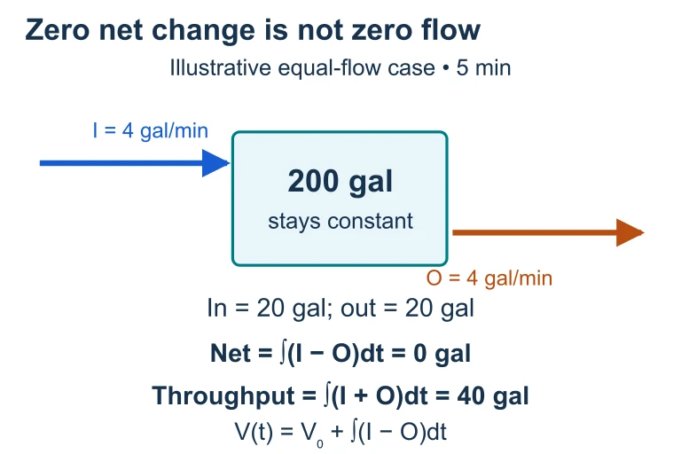Suppose a tank receives and releases 4 gal/min for 5 minutes. Its 200 gal inventory stays constant while 20 gal enters and 20 gal leaves: net change is zero and total throughput is 40 gal.

SECTION 4

Mathematical Framework

FTC Part 1: Differentiating an Accumulation Function

FTC PART 1

d/dx [ ∫ₐˣ f(t) dt ] = f(x)

f must be continuous on an open interval containing [a, x]. The variable of integration t is a dummy variable; the result depends only on the upper limit x.

On the AP exam, the upper limit is often not simply x but a function of x — say g(x). In that case, the chain rule must be applied.

FTC PART 1 WITH CHAIN RULE

d/dx [ ∫ₐ^{g(x)} f(t) dt ] = f(g(x)) · g′(x)

Replace the dummy variable t with the upper limit g(x), then multiply by the derivative of the upper limit. If the lower limit is also a function h(x), subtract: f(g(x))·g′(x) − f(h(x))·h′(x).

FTC Part 2: The Evaluation Theorem

FTC PART 2 (EVALUATION THEOREM)

∫ₐᵇ f(x) dx = F(b) − F(a)

F is any antiderivative of f — that is, F′(x) = f(x). The constant of integration cancels in the subtraction, so you may choose whichever antiderivative is most convenient (typically C = 0).

💡

AP Exam Tip

When asked to evaluate a definite integral, always check whether you can apply FTC Part 2 directly by finding an antiderivative. When asked to find the derivative of an integral with a variable limit, apply FTC Part 1 (with the chain rule if needed). Recognizing which part to use is a frequent source of exam points — and errors.

NET CHANGE THEOREM

∫ₐᵇ F′(x) dx = F(b) − F(a)

This is FTC Part 2 restated: integrating a rate of change over [a, b] yields the net change in the original quantity. For example, if v(t) is velocity, then ∫ₐᵇ v(t) dt = s(b) − s(a), the net displacement.

SECTION 5

Properties and Behavior of Accumulation Functions

Because the AP Calculus BC exam frequently presents graphs of f and asks you to analyze the resulting accumulation function F(x) = ∫ₐˣ f(t) dt, it is essential to understand how features of f translate into features of F. The diagram below summarizes this correspondence, and the table that follows provides a systematic reference.

Left panel: the integrand f(t) with positive area and negative area shown. Right panel: the accumulation function F(x) rises when f > 0, falls when f < 0, and achieves a relative maximum at x = c where f crosses from positive to negative.

Feature of f(t)	Corresponding Feature of F(x)	Reasoning
f(x) > 0	F is increasing	F′(x) = f(x) > 0
f(x) < 0	F is decreasing	F′(x) = f(x) < 0
f(x) = 0 (sign change + → −)	F has a relative maximum	First derivative test: F′ changes from + to −
f(x) = 0 (sign change − → +)	F has a relative minimum	First derivative test: F′ changes from − to +
f is increasing	F is concave up	F″(x) = f′(x) > 0
f is decreasing	F is concave down	F″(x) = f′(x) < 0
f has a local extremum	F has an inflection point	F″ changes sign because f′ changes sign

Translating features of the integrand f into features of the accumulation function F

SECTION 6

Worked Example

Analyzing an Accumulation Function

1
Step 1 — State the Problem

Let g(x) = ∫₁ˣ (3t² − 12) dt. Find g(3), g′(3), and the x-values at which g has a relative minimum on the interval [1, 5].
2
Step 2 — Compute g(3) Using FTC Part 2

We need an antiderivative of 3t² − 12. The antiderivative is t³ − 12t. By the Evaluation Theorem, g(3) = ∫₁³ (3t² − 12) dt = [t³ − 12t]₁³ = (27 − 36) − (1 − 12) = (−9) − (−11) = 2.

g(3) = 2
3
Step 3 — Find g′(3) Using FTC Part 1

By FTC Part 1, g′(x) = 3x² − 12 (we simply substitute x for t in the integrand, since the upper limit is x with no chain rule needed). Therefore, g′(3) = 3(9) − 12 = 27 − 12 = 15.

g′(3) = 15
4
Step 4 — Find Critical Points

Set g′(x) = 0: 3x² − 12 = 0 ⟹ x² = 4 ⟹ x = ±2. On the interval [1, 5], the only critical point is x = 2.
5
Step 5 — Apply the First Derivative Test

Check the sign of g′(x) = 3x² − 12 on either side of x = 2. At x = 1.5: g′(1.5) = 3(2.25) − 12 = 6.75 − 12 = −5.25 < 0. At x = 3: g′(3) = 15 > 0. Since g′ changes from negative to positive at x = 2, g has a relative minimum there.

g has a relative minimum at x = 2
6
Step 6 — Verify with g(2)

For completeness, g(2) = ∫₁² (3t² − 12) dt = [t³ − 12t]₁² = (8 − 24) − (1 − 12) = (−16) − (−11) = −5. So the relative minimum value is −5, confirming that the function dipped below zero before rising back through g(3) = 2.

g(2) = −5 (relative min value)

SECTION 7

Strengths, Common Pitfalls, and Comparisons

Strength	Common Pitfall	How to Avoid It
FTC Part 2 converts limit-of-sums problems into simple antiderivative evaluation.	Forgetting the "+C" when finding a general antiderivative (though it cancels in definite integrals).	For definite integrals, use bracket notation [F(x)]ₐᵇ to make the subtraction explicit.
FTC Part 1 gives an instant derivative without ever finding a closed-form antiderivative.	Neglecting the chain rule when the upper limit is a function g(x) rather than x.	Always write: d/dx [∫ₐ^{g(x)} f(t) dt] = f(g(x)) · g′(x). Train yourself to check the upper limit.
Accumulation functions encode complete information about signed area and can be analyzed with standard derivative tools.	Confusing net signed area (∫ₐᵇ f dx) with total area (∫ₐᵇ \|f\| dx).	Read the problem carefully: 'total distance' requires \|v(t)\|, while 'displacement' or 'net change' requires v(t).
The graph-of-f → features-of-F connection enables rich qualitative reasoning.	Reading F's concavity from f's values instead of f's slope.	Remember: F″ = f′. Concavity of F depends on whether f is increasing or decreasing, not on the sign of f.

Strengths of the FTC paired with the most common student errors

✦

KEY TAKEAWAY

Think of the Fundamental Theorem like a GPS navigation system: your speed at each moment is the integrand f(t), and your odometer reading is the accumulation function F(x). FTC Part 1 says the current speed is the derivative of the odometer reading. FTC Part 2 says you can compute the total trip distance by subtracting odometer readings at the start and end — you do not need to sum every infinitesimal segment by hand. The most common exam error is forgetting to 'multiply by g′(x)' when the upper limit is a function of x — analogous to a GPS that fails to account for how fast the time parameter itself is changing.

SECTION 8

Connections to Advanced Topics

The Fundamental Theorem of Calculus is not merely a computational shortcut — it is the gateway to a vast landscape of advanced mathematics and applications. In AP Calculus BC and beyond, the FTC generalizes in several important directions that you should be aware of, both for exam readiness and for conceptual depth.

FTC Concept	Advanced Generalization	Where It Appears
∫ₐᵇ f(x) dx = F(b) − F(a)	Line integrals of gradient fields: ∫_C ∇F · dr = F(B) − F(A), generalizing FTC to vector calculus (the Gradient Theorem).	Multivariable Calculus, Physics (work-energy theorem)
Net change: ∫ₐᵇ F′(t) dt = F(b) − F(a)	Differential equations: given dy/dx = f(x, y), the solution accumulates change along a solution curve. FTC underpins separation of variables and integral curves.	AP Calculus BC (Topic 7), Engineering
Accumulation function F(x) = ∫ₐˣ f(t) dt	Improper integrals: extending the upper limit to ∞ yields ∫ₐ^∞ f(t) dt = $\lim_{b→∞}$ F(b). Convergence tests build on the FTC.	AP Calculus BC (Topic 6.13), Series convergence
F′(x) = f(x) for continuous f	Lebesgue's theorem: a bounded function on [a, b] is Riemann integrable if and only if it is continuous almost everywhere. The FTC generalizes to the Lebesgue integral.	Real Analysis, Measure Theory

How the FTC generalizes beyond single-variable calculus

For the AP Calculus BC exam, the most immediately relevant extensions are improper integrals and differential equations. In both cases, the Fundamental Theorem provides the bridge: improper integrals are evaluated by applying FTC Part 2 and then taking a limit, while separable differential equations are solved by integrating both sides — an operation justified by the FTC. Understanding the theorem deeply now will make those topics feel like natural extensions rather than isolated techniques.

SECTION 9

Practice Problems

Question 1: CONCEPTUAL

Let F(x) = ∫₂ˣ f(t) dt, where f is continuous on [0, 10]. If f(5) = 0 and f changes sign from positive to negative at t = 5, which of the following must be true?

A. F(5) = 0
B. F has an inflection point at x = 5
C. F has a relative maximum at x = 5
D. F has a relative minimum at x = 5
E. F′(5) is undefined

Show answer (C)

By FTC Part 1, F′(x) = f(x), so F′(5) = f(5) = 0, making x = 5 a critical point. Since f changes from positive to negative at t = 5, F′ changes from positive to negative, so by the First Derivative Test, F has a relative maximum at x = 5. (A) is wrong because F(5) = ∫₂⁵ f(t) dt is the accumulated area from 2 to 5, which need not be zero even though f(5) = 0. (B) is wrong because an inflection point of F requires F″ = f′ to change sign, which would mean f has a local extremum — but the problem states f changes sign, not that f′ changes sign. (D) describes the opposite sign change. (E) is wrong because f is continuous, so F′(5) = f(5) = 0 exists.

Question 2: BASIC CALCULATION

If h(x) = ∫₀^{x²} sin(t) dt, what is h′(x)?

A. sin(x²)
B. 2x · sin(x²)
C. cos(x²) · 2x
D. sin(x²) · 2x + cos(x²)
E. −cos(x²) + 1

Show answer (B)

Apply FTC Part 1 with the chain rule. The upper limit is g(x) = x², so h′(x) = sin(g(x)) · g′(x) = sin(x²) · 2x. (A) omits the chain rule factor of 2x — this is the most common error. (C) incorrectly differentiates sin to cos, confusing the derivative of the antiderivative with the derivative of the integrand. (D) adds an extraneous cos(x²) term. (E) attempts to find the antiderivative of sin(t) and evaluate it, which gives h(x) = −cos(x²) + 1, not h′(x).

Question 3: INTERMEDIATE

Let g(x) = ∫_{2x}^{x³} eᵗ dt. Which of the following gives g′(x)?

A. $e^{x³}$ · 3x² − $e^{2x}$ · 2
B. $e^{x³}$ − $e^{2x}$
C. $e^{x³}$ · 3x² + $e^{2x}$ · 2
D. 3x² $e^{x³}$ − $2e^{2x}$ + C
E. $e^{x³}$ · x³ − $e^{2x}$ · 2x

Show answer (A)

When both limits are functions of x, split using the property: ∫_{h(x)}^{g(x)} f(t) dt = ∫₀^{g(x)} f(t) dt − ∫₀^{h(x)} f(t) dt (or any shared constant). Differentiating: g′(x) = f(g(x)) · g′(x) − f(h(x)) · h′(x) =

e^{x³}

· 3x² −

e^{2x}

· 2. (B) omits both chain rule factors. (C) incorrectly adds the second term instead of subtracting it — recall that differentiating the lower-limit integral introduces a negative sign. (D) includes an arbitrary constant C, which does not appear in derivative expressions. (E) confuses the chain rule factor with the limit itself (writing x³ instead of 3x² and 2x instead of 2).

Question 4: APPLIED

5 pts

A particle moves along the x-axis with velocity v(t) = t² − 4t + 3 for 0 ≤ t ≤ 5. The particle's position at time t = 0 is x(0) = 2. (a) Find the particle's position function x(t). (b) Determine the net displacement of the particle over [0, 5]. (c) Determine the total distance traveled by the particle over [0, 5]. (d) At what time(s) in [0, 5] does the particle change direction? Justify your answer.

Show answer

(a) [1 point] By the FTC, x(t) = x(0) + ∫₀ᵗ v(s) ds = 2 + ∫₀ᵗ (s² − 4s + 3) ds = 2 + [s³/3 − 2s² + 3s]₀ᵗ = 2 + t³/3 − 2t² + 3t. (b) [1 point] Net displacement = ∫₀⁵ v(t) dt = [t³/3 − 2t² + 3t]₀⁵ = (125/3 − 50 + 15) − 0 = 125/3 − 35 = 125/3 − 105/3 = 20/3. (c) [2 points] First find where v(t) = 0: t² − 4t + 3 = (t − 1)(t − 3) = 0, so t = 1 and t = 3. Check signs: v(0) = 3 > 0, v(2) = 4 − 8 + 3 = −1 < 0, v(4) = 16 − 16 + 3 = 3 > 0. Total distance = ∫₀¹ v(t) dt + |∫₁³ v(t) dt| + ∫₃⁵ v(t) dt. Compute each: ∫₀¹ = 1/3 − 2 + 3 = 4/3; ∫₁³ = (9 − 18 + 9) − (1/3 − 2 + 3) = 0 − 4/3 = −4/3; ∫₃⁵ = (125/3 − 50 + 15) − (9 − 18 + 9) = 20/3 − 0 = 20/3. Total distance = 4/3 + 4/3 + 20/3 = 28/3. (d) [1 point] The particle changes direction when v(t) changes sign. v(t) = (t − 1)(t − 3) = 0 at t = 1 and t = 3. Since v changes from positive to negative at t = 1 and from negative to positive at t = 3, the particle changes direction at both t = 1 and t = 3.

Question 5: CRITICAL THINKING

3 pts

Define F(x) = ∫₀ˣ f(t) dt where f is continuous on ℝ and f(t) > 0 for all t. A student claims: "Since f(t) > 0 everywhere, F must be an increasing function on all of ℝ, and therefore F can never equal zero for x > 0." Is the student's reasoning correct? Provide a rigorous justification using the Fundamental Theorem of Calculus.

Show answer

[1 point] The student's claim that F is increasing on all of ℝ is correct. By FTC Part 1, F′(x) = f(x) > 0 for all x, so F is strictly increasing on (−∞, ∞). [1 point] The claim that F(x) ≠ 0 for x > 0 is also correct, and the justification goes further than 'increasing.' Since F(0) = ∫₀⁰ f(t) dt = 0 by definition, and F is strictly increasing (F′ > 0 everywhere), for any x > 0 we have F(x) > F(0) = 0. Therefore F(x) > 0 for all x > 0. [1 point] The student's reasoning is correct in conclusion but could be made more precise. The key logical step is: F(0) = 0 serves as the anchor, and strict monotonicity (guaranteed by FTC Part 1 since f > 0) ensures F(x) > 0 for x > 0 and F(x) < 0 for x < 0. The student should explicitly cite F(0) = 0 and the strict inequality F′ > 0 to complete the argument rigorously.

SUMMARY

Lesson Summary

Summary

The Fundamental Theorem of Calculus establishes the profound inverse relationship between differentiation and integration. FTC Part 1 states that if F(x) = ∫ₐˣ f(t) dt and f is continuous, then F′(x) = f(x) — the derivative of an accumulation function recovers the original integrand. When the upper limit is a composite function g(x), the chain rule must be applied: F′(x) = f(g(x)) · g′(x). FTC Part 2 (the Evaluation Theorem) converts definite integrals into antiderivative subtraction: ∫ₐᵇ f(x) dx = F(b) − F(a), eliminating the need to evaluate limits of Riemann sums.

The accumulation function F(x) = ∫ₐˣ f(t) dt is increasing where f > 0, decreasing where f < 0, has relative extrema where f changes sign, and has inflection points where f has local extrema. The Net Change Theorem — a direct consequence of FTC Part 2 — states that ∫ₐᵇ F′(t) dt = F(b) − F(a), connecting rates of change to total accumulated change. Mastery of these ideas, including the ability to read features of F from the graph of f and to distinguish net accumulation from total accumulation, is essential for both the multiple-choice and free-response sections of the AP Calculus BC exam.