Exponential Models with Differential Equations - AP Calculus BC

SECTION 1

Historical Context & Motivation

The idea that a quantity's rate of change is proportional to its current size is one of the oldest and most powerful principles in mathematics. Long before formal calculus existed, scholars observed that populations, investments, and radioactive substances all seemed to change at rates tied to how much was already present. The exponential model — captured by the differential equation dy/dt = ky — emerged as the unifying framework for all such phenomena. Its elegance lies in the fact that the exponential function is the only non-trivial function that is its own derivative (up to a constant multiple), making it the natural solution to this class of equations.

1614 • Napier's Logarithms

John Napier published tables of logarithms, implicitly encoding exponential relationships and laying groundwork for the constant e.

1683 • Jacob Bernoulli & Compound Interest

While studying compound interest, Bernoulli discovered the limit (1 + 1/n)ⁿ → e ≈ 2.71828, revealing the base of natural exponential growth.

1798 • Malthus's Population Model

Thomas Malthus proposed that unchecked populations grow exponentially — formalized as dP/dt = kP — sparking debates on resource limits.

1902 • Rutherford & Soddy's Decay Law

Ernest Rutherford and Frederick Soddy demonstrated that radioactive decay follows dN/dt = −λN, introducing the concept of half-life.

The recurring question across all these domains is deceptively simple: if a quantity changes at a rate proportional to itself, what function describes that quantity over time? Answering this question requires solving a separable differential equation — a technique central to AP Calculus BC and foundational to modeling in physics, biology, economics, and chemistry.

SECTION 2

Core Principles & Definitions

Exponential models arise whenever a differential equation states that the instantaneous rate of change of a quantity is directly proportional to the quantity itself. Understanding this model requires command of several interconnected ideas, from the structure of the equation to the interpretation of its parameters.

The Differential Equation dy/dt = ky

The rate of change of y with respect to t is proportional to y. The constant k is the relative growth rate (units: per time). When k > 0 the model describes growth; when k < 0 it describes decay.

General Solution: y = Ceᵏᵗ

Separation of variables yields y(t) = Ce^kt, where C is the initial value y(0). This is the unique family of solutions.

Initial Condition y(0) = y₀

The initial condition pins down the arbitrary constant C, giving the particular solution y(t) = y₀e^kt. Every exponential model requires this anchor point.

Doubling Time & Half-Life

For growth (k > 0), the doubling time is ln 2 / k. For decay (k < 0), the half-life is ln 2 / |k|. Both are independent of the initial amount.

✦

KEY TAKEAWAY

Think of an exponential process like a snowball rolling downhill: the bigger it gets, the faster it picks up more snow — and that faster rate makes it grow even bigger. The differential equation dy/dt = ky captures exactly this self-reinforcing feedback. The function e^kt is the mathematical fingerprint of any process where the rate of change is proportional to the current state.

SECTION 3

Visualizing Exponential Growth & Decay

The graph below illustrates two solution curves for the differential equation dy/dt = ky sharing the same initial value y₀ = 2. The green curve shows exponential growth (k = 0.5), while the pink curve shows exponential decay (k = −0.5). Notice how both curves pass through the same initial point but diverge dramatically — the growth curve accelerates upward while the decay curve approaches the horizontal asymptote y = 0 from above but never reaches it.

Both curves share the initial value y₀ = 2 (gold dot). The growth curve (k > 0) increases without bound, while the decay curve (k < 0) approaches the horizontal asymptote y = 0 but never crosses it.

Several features are worth noting. First, both curves are concave in a characteristic way: the growth curve is concave up (since y'' = k²y > 0 when k > 0), while the decay curve is also concave up (since y'' = k²y > 0 for y > 0 regardless of the sign of k). Second, the rate of change at any point on either curve equals k times the y-value at that point — a fact you can verify by drawing a tangent line and estimating its slope.

SECTION 4

Mathematical Framework

The derivation of the exponential model from the differential equation dy/dt = ky is a textbook application of separation of variables. This technique is one of the first and most important methods for solving ordinary differential equations, and the exponential equation provides the cleanest possible illustration.

THE DIFFERENTIAL EQUATION

dy/dt = ky

y = y(t) is the unknown function, t is the independent variable (often time), and k is a nonzero real constant.

SEPARATION OF VARIABLES

(1/y) dy = k dt

Divide both sides by y (assuming y ≠ 0) and multiply by dt to isolate all y-terms on the left and all t-terms on the right.

INTEGRATION

ln|y| = kt + C₁

Integrate both sides: ∫(1/y) dy = ∫k dt. The left side yields ln|y| and the right side yields kt + C₁, where C₁ is the constant of integration.

GENERAL SOLUTION

y(t) = Ce^(kt), where C = y(0)

Exponentiate both sides: |y| = $e^{kt + C₁}$ = $e^{C₁}$ · $e^{kt}$ . Setting C = ± $e^{C₁}$ (which also absorbs the case y > 0 or y < 0), we obtain y = $Ce^{kt}$ . Applying the initial condition y(0) = y₀ gives C = y₀.

💡

Why y = 0 is not lost

We divided by y during separation, which assumes y ≠ 0. However, y(t) = 0 for all t is indeed a solution (simply substitute into dy/dt = ky). It corresponds to the particular solution with C = 0. So the general solution y = Ce^kt for C ∈ ℝ captures every solution, including the trivial one.

A steaming coffee cup and a cool liquid cup with condensation, each probed, with a shared room-reference probe between them. With ambient temperature 22 °C and k > 0, T′ = −k(T − 22). A warmer liquid cools and a cooler liquid warms, both approaching ambient temperature.

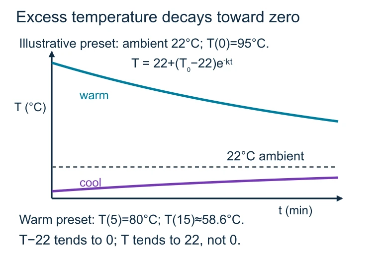With ambient temperature 22 °C and k > 0, T′ = −k(T − 22). A warmer liquid cools and a cooler liquid warms, both approaching ambient temperature.

SECTION 5

Applications & Classification

The equation dy/dt = ky appears across virtually every scientific discipline. The sign of k and the physical interpretation of y give rise to a taxonomy of classic models, each with its own terminology and conventions. The diagram below maps common applications to their place on the growth–decay spectrum and highlights the key derived quantities — doubling time and half-life — that appear on the AP exam.

Common applications of dy/dt = ky organized by the sign of k. Decay models (k < 0) appear on the left; growth models (k > 0) on the right. The gold box highlights the universal doubling-time and half-life formulas.

Application	Equation Form	Sign of k	Derived Quantity
Bacterial growth	dP/dt = rP	r > 0	Doubling time = ln 2 / r
Radioactive decay	dN/dt = −λN	−λ < 0	Half-life = ln 2 / λ
Continuous compounding	dA/dt = rA	r > 0	Doubling time = ln 2 / r
Newton's cooling (transformed)	du/dt = −ku	−k < 0	Time to halve temp diff = ln 2 / k

Summary of common exponential models tested on AP Calculus BC

SECTION 6

Worked Example

A sample of a radioactive isotope has a mass of 80 grams at time t = 0. After 3 hours, only 50 grams remain. Find the decay constant k, write the particular solution, and determine the half-life of the isotope.

Radioactive Decay Problem

1
Step 1 — Set Up the Differential Equation

Radioactive decay obeys dy/dt = ky with k < 0. The general solution is y(t) = y₀e^kt. We are given y₀ = 80 g, so y(t) = 80e^kt.

y(t) = $80e^{kt}$
2
Step 2 — Apply the Second Condition to Find k

We know y(3) = 50. Substituting: 50 = 80e^3k. Divide both sides by 80: e^3k = 50/80 = 5/8. Take the natural logarithm: 3k = ln(5/8). Therefore k = ln(5/8) / 3.

k = ln(5/8) / 3 ≈ −0.1567 per hour
3
Step 3 — Write the Particular Solution

Substituting the value of k back into the general solution gives the particular solution for this isotope.

y(t) = $80e^{−0.1567t}$ grams
4
Step 4 — Compute the Half-Life

The half-life t₁/₂ satisfies y(t₁/₂) = y₀/2, which gives e^k·t₁/₂ = 1/2. Solving: t₁/₂ = ln(2) / |k| = ln(2) / 0.1567.

t₁/₂ = ln 2 / 0.1567 ≈ 4.42 hours
5
Step 5 — Verify

At t = 4.42: y(4.42) = 80e^{−0.1567 × 4.42} = 80e^−0.6926 ≈ 80 × 0.5003 ≈ 40.0 g, which is half of 80. ✓

Confirmed: half the initial mass remains at t ≈ 4.42 hr

SECTION 7

Strengths & Limitations of the Exponential Model

The exponential model is remarkably powerful for short-to-medium time horizons, but it has well-known limitations that motivate more sophisticated models such as logistic growth. Understanding when the model applies — and when it breaks down — is essential for both the AP exam and real-world modeling.

Strengths	Limitations
Exact closed-form solution y = y₀ $e^{kt}$ is easily evaluated and differentiated.	Unbounded growth (k > 0) is unrealistic for populations facing limited resources.
Only two parameters (y₀ and k) make the model easy to fit from two data points.	Assumes a constant relative growth rate — cannot capture changing conditions.
Universality: applies to any proportional-rate phenomenon (physics, chemistry, finance).	Sensitive to the value of k: small errors in k produce large errors over long time horizons.
Serves as the linearized approximation of more complex models near equilibrium.	Does not model carrying capacity, threshold effects, or periodic behavior.

Strengths vs. Limitations of dy/dt = ky

✦

KEY TAKEAWAY

The exponential model is like a first-order Taylor polynomial for growth processes — it gives an excellent local approximation, but its predictions diverge from reality over long intervals. That is precisely why the AP curriculum follows exponential models with logistic models (dy/dt = ky(1 − y/L)), which introduce a carrying capacity L to correct for resource saturation.

SECTION 8

Connection to Advanced Theory

The exponential differential equation dy/dt = ky is the simplest autonomous first-order ODE, and it serves as the gateway to a rich landscape of more advanced models. On the AP Calculus BC exam, the exponential model is often contrasted with the logistic model, and understanding their differences is frequently tested. Beyond the AP course, this equation reappears in linear systems of ODEs, Laplace transforms, and even quantum mechanics.

Feature	Exponential: dy/dt = ky	Logistic: dy/dt = ky(1 − y/L)
Growth rate	Proportional to y (constant per-capita rate)	Proportional to y(1 − y/L); slows as y → L
Long-term behavior (k > 0)	y → ∞ (unbounded)	y → L (carrying capacity)
Equilibria	Only y = 0	y = 0 (unstable) and y = L (stable)
Solution form	y = y₀ $e^{kt}$	y = L / (1 + $Ae^{−kt}$ ), A = (L − y₀)/y₀
Inflection point	None (always concave up for y > 0)	At y = L/2 (maximum growth rate)

Exponential vs. Logistic — a comparison frequently tested on AP Calculus BC

In more advanced courses, the scalar equation dy/dt = ky generalizes to the matrix equation dx⃗/dt = Ax⃗, where solutions involve matrix exponentials and eigenvalues. The eigenvalues of A play the same role as k: positive real parts indicate instability (growth), and negative real parts indicate stability (decay). Mastering the scalar case now builds the intuition needed for these higher-dimensional systems.

SECTION 9

Practice Problems

Question 1: CONCEPTUAL

If a quantity y satisfies dy/dt = ky with k < 0 and y(0) > 0, which of the following statements is true about y(t) for all t > 0? (A) y(t) is negative and decreasing (B) y(t) is positive and increasing (C) y(t) is positive, decreasing, and concave up (D) y(t) is positive, decreasing, and concave down (E) y(t) eventually equals zero at some finite time

A. y(t) is negative and decreasing
B. y(t) is positive and increasing
C. y(t) is positive, decreasing, and concave up
D. y(t) is positive, decreasing, and concave down
E. y(t) eventually equals zero at some finite time

Show answer (C)

Correct: (C). Since y(0) > 0 and y(t) = y₀

e^{kt}

with k < 0, the exponential is always positive (eliminating A and E). The function is decreasing because dy/dt = ky < 0 when y > 0 and k < 0 (eliminating B). For concavity, y'' = k²y > 0 for all y > 0, so the curve is concave up (eliminating D). The solution approaches zero asymptotically but never reaches it in finite time (eliminating E).

Question 2: BASIC CALCULATION

A bacteria population grows according to dP/dt = 0.03P, where P is measured in thousands and t in hours. If P(0) = 5 (thousand), what is the population at t = 10 hours? (A)

5e^{0.3}

≈ 6.75 thousand (B)

5e^{3}

≈ 100.4 thousand (C) 5 + 0.03(10) = 5.3 thousand (D) 5

(0.03)^{10}

thousand (E)

e^{0.3}

≈ 1.35 thousand

A. $5e^{0.3}$ ≈ 6.75 thousand
B. $5e^{3}$ ≈ 100.4 thousand
C. 5 + 0.03(10) = 5.3 thousand
D. 5 $(0.03)^{10}$ thousand
E. $e^{0.3}$ ≈ 1.35 thousand

Show answer (A)

Correct: (A). The general solution is P(t) = P₀

e^{kt}

5e^{0.03t}

. At t = 10: P(10) =

5e^{0.03 × 10}

5e^{0.3}

≈ 5 × 1.3499 ≈ 6.75 thousand. (B) incorrectly uses k = 0.3 instead of 0.03. (C) applies a linear model, not exponential. (D) raises the rate to the 10th power, which is meaningless here. (E) omits the initial value y₀ = 5.

Question 3: INTERMEDIATE

A substance decays so that 60% of its original amount remains after 4 years. What is the half-life of the substance? (A) 4 ln 2 / ln(5/3) (B) ln 2 / 4 (C) 4 ln(5/3) / ln 2 (D) 4 / ln(5/3) (E) 4 ln 2

A. 4 ln 2 / ln(5/3)
B. ln 2 / 4
C. 4 ln(5/3) / ln 2
D. 4 / ln(5/3)
E. 4 ln 2

Show answer (A)

Correct: (A). We have y(4) = 0.6 y₀, so

e^{4k}

= 0.6 = 3/5, giving k = ln(3/5)/4 = −ln(5/3)/4. The half-life is t₁/₂ = ln 2 / |k| = ln 2 / (ln(5/3)/4) = 4 ln 2 / ln(5/3). (B) would require k = −1, which doesn't match the data. (C) inverts the fraction inside the logarithm relative to ln 2. (D) omits the ln 2 factor entirely. (E) incorrectly assumes |k| = 1/4.

Question 4: APPLIED

4 pts

A cup of coffee is brewed at 95°C and placed in a room at 20°C. After 5 minutes, its temperature is 70°C. Using Newton's Law of Cooling — which states that the temperature difference u(t) = T(t) − 20 satisfies du/dt = −ku — find the temperature of the coffee at t = 12 minutes. Show all work.

Show answer

Point 1 — Set up the model (1 pt): Let u(t) = T(t) − 20. Then u(0) = 95 − 20 = 75 and u(5) = 70 − 20 = 50. The solution is u(t) =

75e^{−kt}

. Point 2 — Find k (1 pt): 50 =

75e^{−5k}

→

e^{−5k}

= 2/3 → −5k = ln(2/3) → k = −ln(2/3)/5 = ln(3/2)/5 ≈ 0.08109. Point 3 — Evaluate u(12) (1 pt): u(12) =

75e^{−0.08109 × 12}

75e^{−0.9731}

≈ 75 × 0.3785 ≈ 28.39°C. Point 4 — Convert back to temperature (1 pt): T(12) = u(12) + 20 ≈ 28.39 + 20 = 48.39°C ≈ 48.4°C.

Question 5: CRITICAL THINKING

3 pts

A quantity y satisfies dy/dt = ky with y(0) = A > 0. Prove that if the quantity triples every T units of time — i.e., y(T) = 3A — then y(t) can be rewritten in the form y(t) = A ·

3^{t/T}

, and determine the relationship between k and T.

Show answer

Point 1 — Apply the condition y(T) = 3A (1 pt): From y(t) =

Ae^{kt}

, setting t = T: 3A =

Ae^{kT}

→

e^{kT}

= 3 → kT = ln 3 → k = ln 3 / T. Point 2 — Rewrite the solution (1 pt): Substituting k = ln 3 / T: y(t) =

Ae^{(ln 3 / T)·t}

= A ·

e^{ln 3 · t/T}

= A ·

(e^{ln 3})^{t/T}

= A ·

3^{t/T}

. Point 3 — State the relationship (1 pt): The continuous growth rate k and the tripling time T are related by k = ln 3 / T, or equivalently T = ln 3 / k. This generalizes: if y multiplies by a factor m every T units, then k = ln m / T. The doubling-time formula (k = ln 2 / T) and half-life formula are special cases.

SUMMARY

Lesson Summary

Summary

The exponential model arises from the differential equation dy/dt = ky, which states that a quantity's rate of change is proportional to its current value. Solving by separation of variables yields the general solution y(t) = y₀ $e^{kt}$ , where y₀ is the initial value and k is the continuous relative growth (k > 0) or decay (k < 0) rate.

Key derived quantities include the doubling time (ln 2 / k for growth) and half-life (ln 2 / |k| for decay), both independent of y₀. Applications span population dynamics, radioactive decay, compound interest, and Newton's Law of Cooling. While powerful and elegant, the model's assumption of constant per-capita rate limits its long-term accuracy, motivating the logistic model as the natural next step in the AP Calculus BC curriculum.