Exploring Accumulations of Change - AP Calculus BC

SECTION 1

Historical Context & Motivation

The question of how to recover a total quantity from knowledge of its instantaneous rate of change is one of the oldest in mathematics. Ancient Greek geometers understood that the area of a circle could be approximated by summing the areas of inscribed polygons with ever more sides, an idea that foreshadowed the limiting processes central to integral calculus. Centuries later, mathematicians in medieval India and the Islamic world developed early summation formulas for powers of integers, tools that would prove essential for computing areas under curves. The decisive breakthrough came in seventeenth-century Europe, when Isaac Newton and Gottfried Wilhelm Leibniz independently formalized the inverse relationship between differentiation and integration, giving rise to the Fundamental Theorem of Calculus. This theorem unified two seemingly distinct problems—finding tangent lines and computing areas—into a single coherent framework that remains the backbone of modern analysis.

~250 BCE • Archimedes' Method of Exhaustion

Archimedes approximated the area of a parabolic segment by summing an infinite geometric series of triangular slices, anticipating the concept of an integral as the limit of a sum.

1635 • Cavalieri's Principle

Bonaventura Cavalieri published Geometria indivisibilibus, using 'indivisibles' to compare areas and volumes—an early systematic approach to accumulation via infinitesimal slices.

1668 • Newton's Fluxions

Newton developed the method of fluxions and fluents, recognizing that the area under a rate-of-change curve could be recovered by reversing differentiation.

1684 • Leibniz Publishes Integral Notation

Leibniz introduced the elongated 'S' symbol ∫ and the dx notation, giving calculus a powerful symbolic language still in use today.

1854 • Riemann's Formalization

Bernhard Riemann provided a rigorous definition of the definite integral using partitioned sums and limits, placing accumulation of change on solid theoretical ground.

The central question this lesson addresses is deceptively simple: if you know how fast a quantity is changing at every instant, how do you determine the total change over an interval? Whether the quantity is distance, population, charge, or revenue, the answer lies in the concept of accumulation—the process of summing infinitely many infinitesimal contributions to obtain a finite total.

SECTION 2

Core Principles & Definitions

At the heart of integration lies the idea that a definite integral computes the net accumulation of a quantity over an interval by aggregating its rate of change. Before diving into computation techniques, it is essential to internalize the foundational concepts that give the integral its meaning and power. The following four principles form the conceptual backbone of every accumulation problem you will encounter on the AP Calculus BC exam, from straightforward area calculations to sophisticated applications involving particle motion and differential equations.

Rate × Time = Accumulation

If f(t) represents a rate of change, then the product f(t) · Δt approximates the change in the quantity over a small interval Δt. Summing many such products over [a, b] and taking the limit as Δt → 0 yields the definite integral ∫ from a to b of f(t) dt.

Signed Area Interpretation

The definite integral ∫ₐᵇ f(x) dx equals the net signed area between the graph of f and the x-axis. Regions above the axis contribute positive area, while regions below contribute negative area. This signed interpretation is crucial for understanding net versus total accumulation.

Riemann Sums as Approximations

A Riemann sum partitions [a, b] into n subintervals, evaluates f at a sample point in each, and sums the resulting products f(xₖ*) · Δxₖ. As the partition becomes finer (n → ∞ and max Δxₖ → 0), the Riemann sum converges to the definite integral.

Accumulation Function

The function F(x) = ∫ₐˣ f(t) dt defines the accumulated value from a fixed starting point a to a variable endpoint x. By the Fundamental Theorem of Calculus (Part 1), F′(x) = f(x), revealing that the rate of change of accumulated quantity equals the integrand.

✦

KEY TAKEAWAY

Think of integration as a sophisticated odometer. Just as a car's odometer accumulates distance by continuously tracking speed over time, the definite integral accumulates any quantity by continuously summing its rate of change. If the car reverses, the odometer (in a signed sense) subtracts distance—mirroring how negative rate values reduce the net integral. The integral is not merely an area formula; it is the universal tool for converting 'how fast' into 'how much.'

SECTION 3

Visualizing Accumulation with Riemann Sums

The transition from a discrete sum to a continuous integral is best understood visually. The diagram below illustrates how a Riemann sum approximates the area under a curve f(x) = −0.08x² + 2.5x on the interval [1, 8]. Each rectangle's height is determined by the function value at the left endpoint of its subinterval, and the total area of all rectangles approximates the definite integral. As the number of rectangles increases, the approximation improves and converges to the exact accumulated value.

The violet rectangles represent the left Riemann sum with n = 7 equal subintervals on [1, 8]. The cyan curve is f(x) = −0.08x² + 2.5x. The sum of rectangle areas approximates ∫₁⁸ f(x) dx. Notice that some rectangles overshoot and some undershoot the curve—these errors diminish as n → ∞.

Observe that the rectangles provide a piecewise-constant approximation of f. Where f is increasing, left-endpoint rectangles underestimate the true area; where f is decreasing, they overestimate. This systematic pattern of over- and under-approximation motivates the use of midpoint and trapezoidal rules for improved accuracy, topics you will revisit in the numerical integration unit. The key insight here is that as Δx → 0 (equivalently, n → ∞), every Riemann sum converges to the same value—the definite integral—regardless of whether you choose left, right, or midpoint sample points, provided f is integrable on the interval.

SECTION 4

Mathematical Framework

The rigorous mathematical machinery behind accumulation rests on three pillars: the formal definition of the definite integral via Riemann sums, and the two parts of the Fundamental Theorem of Calculus (FTC). Together, these results transform the conceptually intuitive idea of 'summing rates to get totals' into a precise computational tool.

DEFINITE INTEGRAL AS A LIMIT OF RIEMANN SUMS

∫ₐᵇ f(x) dx = lim (n→∞) Σₖ₌₁ⁿ f(xₖ*) · Δx

Here Δx = (b − a)/n, xₖ* is any sample point in the k-th subinterval [xₖ₋₁, xₖ], and the limit is taken as the norm of the partition tends to zero. This definition gives meaning to the integral for any Riemann-integrable function f on [a, b].

FTC PART 1 — THE ACCUMULATION FUNCTION

If F(x) = ∫ₐˣ f(t) dt, then F′(x) = f(x)

This states that the derivative of the accumulation function equals the integrand. It guarantees that every continuous function f has an antiderivative, namely the accumulation function F(x). When the upper limit is a composite function g(x), the chain rule gives d/dx [∫ₐᵍ⁽ˣ⁾ f(t) dt] = f(g(x)) · g′(x).

FTC PART 2 — EVALUATION THEOREM

∫ₐᵇ f(x) dx = F(b) − F(a), where F′(x) = f(x)

If F is any antiderivative of f on [a, b], then the definite integral equals the net change in F. This transforms integration from an infinite limiting process into simple antiderivative evaluation, making exact computation feasible.

NET CHANGE THEOREM

∫ₐᵇ f′(x) dx = f(b) − f(a)

A direct consequence of FTC Part 2: the integral of a rate of change over [a, b] equals the net change in the original quantity. For example, if v(t) is velocity, then ∫ₐᵇ v(t) dt gives the net displacement, while ∫ₐᵇ |v(t)| dt gives the total distance traveled.

A subtle but exam-critical distinction exists between net change and total accumulation. The integral ∫ₐᵇ f(t) dt computes the net (signed) accumulation—positive and negative contributions may partially cancel. If the problem asks for total accumulation in the unsigned sense (e.g., total distance rather than displacement), you must integrate the absolute value |f(t)|. On the AP exam, reading the problem statement carefully to distinguish these two cases is essential for full credit.

A stirred transparent tank has one upper inlet and one lower outlet with a valve. The exact diagram links its 100 L salt balance to a computed approach to equilibrium. Suppose a tank receives and releases 4 gal/min for 5 minutes. Its 200 gal inventory stays constant while 20 gal enters and 20 gal leaves: net change is zero and total throughput is 40 gal.

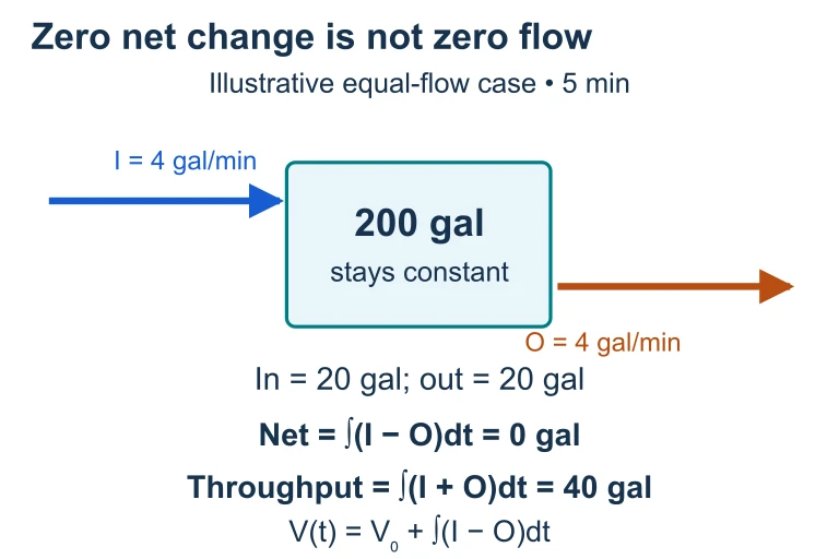Suppose a tank receives and releases 4 gal/min for 5 minutes. Its 200 gal inventory stays constant while 20 gal enters and 20 gal leaves: net change is zero and total throughput is 40 gal.

SECTION 5

Riemann Sum Types & Approximation Strategies

When an antiderivative is unavailable in closed form—or when f is given only as a table of values—approximation methods become indispensable. The AP Calculus BC exam frequently tests your ability to set up and evaluate left Riemann sums, right Riemann sums, midpoint sums, and the trapezoidal rule from tabular data. Understanding when each method over- or underestimates the true integral—based on the monotonicity and concavity of f—is a recurring theme in both multiple-choice and free-response questions.

Four common Riemann sum methods applied to an increasing function. The violet rectangles (left sum) underestimate, the pink rectangles (right sum) overestimate, and the green midpoint rectangles generally provide the closest approximation. The amber trapezoids average the left and right estimates. The concavity of f determines whether the trapezoidal rule overestimates or underestimates.

Method	Formula (equal subintervals)	Overestimates when…	Underestimates when…
Left Riemann	Σ f(xₖ₋₁) · Δx	f is decreasing	f is increasing
Right Riemann	Σ f(xₖ) · Δx	f is increasing	f is decreasing
Midpoint	Σ f((xₖ₋₁ + xₖ)/2) · Δx	f is concave up	f is concave down
Trapezoidal	(Δx/2)[f(x₀) + 2f(x₁) + … + 2f(xₙ₋₁) + f(xₙ)]	f is concave up	f is concave down

Summary of Riemann sum methods and their estimation behavior

SECTION 6

Worked Example: Accumulation from a Rate Table

A water tank is being filled at a variable rate. The table below gives the rate of water flow, R(t), in liters per minute, at selected times t (in minutes). Use a left Riemann sum with three subintervals to approximate the total volume of water that enters the tank from t = 0 to t = 12.

t (min)	0	3	7	12
R(t) (L/min)	4.0	7.2	6.1	3.5

Rate of water flow at selected times

Left Riemann Sum from Tabular Data

1
Step 1 — Identify the subintervals

The data points divide [0, 12] into three subintervals: [0, 3], [3, 7], and [7, 12]. Note that these subintervals have unequal widths: Δt₁ = 3 − 0 = 3, Δt₂ = 7 − 3 = 4, and Δt₃ = 12 − 7 = 5.

Subintervals: [0, 3], [3, 7], [7, 12] with widths 3, 4, 5
2
Step 2 — Apply left-endpoint values

For a left Riemann sum, we use the function value at the left endpoint of each subinterval. Thus we use R(0) = 4.0 for the first subinterval, R(3) = 7.2 for the second, and R(7) = 6.1 for the third.

Left-endpoint values: 4.0, 7.2, 6.1
3
Step 3 — Compute each product R(tₖ) · Δtₖ

Each product represents the approximate volume of water entering during that subinterval: R(0) · Δt₁ = 4.0 × 3 = 12.0 L; R(3) · Δt₂ = 7.2 × 4 = 28.8 L; R(7) · Δt₃ = 6.1 × 5 = 30.5 L.

Products: 12.0, 28.8, 30.5
4
Step 4 — Sum to obtain the approximation

The left Riemann sum is the total of these products: 12.0 + 28.8 + 30.5 = 71.3 liters. This approximates ∫₀¹² R(t) dt, the total volume of water that entered the tank over the 12-minute period. Because the subintervals have unequal widths, each term carries a different weight in the sum—a common feature of AP exam tabular problems.

Left Riemann Sum ≈ 71.3 liters

💡

AP Exam Tip

When data is given in a table with unequal spacing, you must use the actual Δt values for each subinterval—not a uniform width. Many students lose points by assuming equal subintervals. Always write out each product R(tₖ) · Δtₖ explicitly to earn full credit on free-response questions.

SECTION 7

Net Change vs. Total Accumulation

One of the most common sources of error on the AP exam is confusing net change with total accumulation. Consider a particle moving along a line with velocity v(t). The integral ∫ₐᵇ v(t) dt gives the net displacement—the difference between the particle's final and initial positions—because intervals where v(t) < 0 (the particle moves backward) contribute negatively. By contrast, the integral ∫ₐᵇ |v(t)| dt gives the total distance traveled, treating all motion as positive regardless of direction. The table below clarifies this critical distinction across multiple contexts.

Context	Rate Function f(t)	∫ₐᵇ f(t) dt gives…	∫ₐᵇ \|f(t)\| dt gives…
Particle motion	Velocity v(t)	Net displacement	Total distance traveled
Population change	Growth rate P′(t)	Net population change	Total absolute change
Economics	Revenue rate R′(t)	Net revenue change	Total revenue movement
Fluid flow	Flow rate Q(t)	Net volume gained	Total volume that flowed

Net change vs. total accumulation in different contexts

✦

KEY TAKEAWAY

Imagine tracking your bank account balance over a month. Some days you earn money (positive rate), and some days you spend (negative rate). The integral of your income rate gives the net change in your balance—how much richer or poorer you are at month's end. But if you want to know the total amount of money that moved through your account (the sum of all deposits and withdrawals), you integrate the absolute value of the rate. On the AP exam, the words 'net,' 'total distance,' and 'total change' are precise signals that determine which integral to set up.

SECTION 8

Connections to Advanced Topics

The idea of accumulation extends well beyond basic area computations. On the AP Calculus BC exam, accumulation functions appear in contexts ranging from differential equations to parametric and polar area to series convergence. Each of these advanced topics is, at its core, an application of accumulating infinitesimal changes. The table below maps the foundational accumulation concepts from this lesson to their advanced counterparts that you will encounter later in the course.

Foundation (This Lesson)	Advanced Extension (BC Topics)	Key Connection
∫ₐᵇ f(x) dx as net area	Area in polar: ½∫ₐᵇ [r(θ)]² dθ	Accumulation of infinitesimal sector areas
Riemann sums → definite integral	Euler's method for dy/dx = f(x, y)	Discrete stepping approximates continuous accumulation
FTC: d/dx ∫ₐˣ f(t) dt = f(x)	Solving IVPs: y = y₀ + ∫ₐˣ f(t, y(t)) dt	Initial value + accumulated change = current value
∫ₐᵇ \|v(t)\| dt (total distance)	Arc length: ∫ₐᵇ √(1 + [f′(x)]²) dx	Accumulating infinitesimal distances along a curve
Convergent Riemann sums	Integral test for series: Σ aₙ vs. ∫₁∞ f(x) dx	Improper integrals govern series convergence

From foundational accumulation to BC-level applications

As you progress through the BC curriculum, notice that every new integral formula—whether for arc length, surface area of revolution, or work done by a variable force—follows the same template: identify the quantity being accumulated, express an infinitesimal contribution (the integrand times dx, dt, or dθ), and sum over the relevant interval. Mastering the conceptual framework of accumulation now will make every subsequent topic feel like a natural extension rather than an isolated technique.

SECTION 9

Practice Problems

Question 1: CONCEPTUAL

A particle moves along the x-axis with velocity v(t) for 0 ≤ t ≤ 10. If v(t) > 0 for 0 < t < 6 and v(t) < 0 for 6 < t < 10, which of the following correctly describes the relationship between the particle's displacement and total distance traveled over [0, 10]?

A. Displacement equals total distance because the integral accounts for direction.
B. Displacement is greater than total distance because the particle moved forward more than backward.
C. Total distance traveled is greater than or equal to the absolute value of displacement.
D. Total distance traveled equals −∫₀¹⁰ v(t) dt because the particle reverses direction.
E. It is impossible to compare displacement and total distance without knowing the exact formula for v(t).

Show answer (C)

C is correct. Displacement = ∫₀¹⁰ v(t) dt (a signed quantity), while total distance = ∫₀¹⁰ |v(t)| dt. Since |v(t)| ≥ v(t) for all t (with strict inequality when v(t) < 0), the total distance is always ≥ |displacement|. (A) is wrong because displacement is net/signed while total distance is unsigned—they differ whenever the particle reverses. (B) confuses the relationship; displacement can be less than total distance even if the particle spent more time moving forward. (D) incorrectly negates the integral; total distance requires the absolute value, not a negation. (E) is incorrect because the inequality total distance ≥ |displacement| holds generally, without needing the explicit formula.

Question 2: BASIC CALCULATION

The rate of water flowing into a tank is given by R(t) = 3t² + 2 liters per minute. How many liters of water enter the tank from t = 1 to t = 4 minutes?

A. 63 liters
B. 66 liters
C. 69 liters
D. 72 liters
E. 75 liters

Show answer (C)

C is correct. We compute ∫₁⁴ (3t² + 2) dt = [t³ + 2t]₁⁴ = (64 + 8) − (1 + 2) = 72 − 3 = 69 liters. (A) 63 would result from incorrectly evaluating the antiderivative (e.g., omitting the 2t term). (B) 66 might arise from an arithmetic error in subtraction. (D) 72 represents only F(4) without subtracting F(1). (E) 75 could result from evaluating from t = 0 instead of t = 1 or from a power rule error.

Question 3: INTERMEDIATE

Let g(x) = ∫₂ˣ (t² − 4t + 3) dt. At which value of x does g have a relative minimum?

A. x = 1
B. x = 2
C. x = 3
D. x = 4
E. g has no relative minimum

Show answer (C)

C is correct. By FTC Part 1, g′(x) = x² − 4x + 3 = (x − 1)(x − 3). Setting g′(x) = 0 gives x = 1 and x = 3. To classify, check the sign of g′: for 1 < x < 3, g′(x) < 0 (g is decreasing), and for x > 3, g′(x) > 0 (g is increasing). Since g changes from decreasing to increasing at x = 3, g has a relative minimum there. (A) x = 1 is where g′ = 0 but the sign changes from positive to negative, giving a relative maximum. (B) x = 2 is the lower limit of integration where g(2) = 0, but g′(2) = 4 − 8 + 3 = −1 ≠ 0, so it is not a critical point. (D) x = 4 gives g′(4) = 3 > 0, which is not a critical point. (E) is incorrect since we demonstrated a relative minimum at x = 3.

Question 4: APPLIED

5 pts

A factory's rate of production of a chemical compound is modeled by P(t) =

50e^{−0.1t}

kilograms per hour, where t is measured in hours since the start of a production shift. (a) Write, but do not evaluate, an integral expression that gives the total mass of compound produced during the first 8 hours. (b) Evaluate the integral from part (a) to find the total mass produced, to the nearest kilogram. (c) Using a left Riemann sum with four equal subintervals, approximate the integral from part (a). Show the computations that lead to your answer. (d) Is the approximation in part (c) an overestimate or an underestimate of the actual total mass produced? Justify your answer.

Show answer

Rubric (5 points): (a) [1 point] The integral expression is ∫₀⁸

50e^{−0.1t}

dt. Award 1 point for correct integrand, correct limits, and correct variable of integration. (b) [1 point] Antiderivative: ∫

50e^{−0.1t}

dt = 50 · (−10)

e^{−0.1t}

= −

500e^{−0.1t}

. Evaluating: [−

500e^{−0.1t}

]₀⁸ = −

500e^{−0.8}

− (−500e⁰) = −500(0.44933) + 500 = 500 − 224.664 = 275.336 ≈ 275 kilograms. Award 1 point for correct antiderivative evaluation and final numerical answer. (c) [2 points] With four equal subintervals on [0, 8], Δt = 2. Left endpoints: t = 0, 2, 4, 6. P(0) = 50e⁰ = 50 P(2) =

50e^{−0.2}

≈ 40.937 P(4) =

50e^{−0.4}

≈ 33.516 P(6) =

50e^{−0.6}

≈ 27.441 Left Riemann Sum = 2(50 + 40.937 + 33.516 + 27.441) = 2(151.894) ≈ 303.788 kg. Award 1 point for correct setup (identifying Δt = 2 and left endpoints). Award 1 point for correct computation of the sum. (d) [1 point] P(t) =

50e^{−0.1t}

is a decreasing function (since P′(t) = −

5e^{−0.1t}

< 0). For a decreasing function, the left Riemann sum uses function values that are larger than the function's values over the rest of each subinterval, so the left Riemann sum is an overestimate. Award 1 point for correct conclusion with valid justification referencing the decreasing nature of P.

Question 5: CRITICAL THINKING

3 pts

Let f be a continuous function on [0, 10] and define F(x) = ∫₀ˣ f(t) dt. Suppose F(3) = 7, F(7) = 7, and f(5) = 0 with f(x) > 0 for 0 < x < 5 and f(x) < 0 for 5 < x < 10. (a) Explain why F has an absolute maximum on [0, 10] at x = 5. (b) Find the value of ∫₃⁷ f(t) dt and interpret its meaning in terms of the graph of f. (c) Must there exist a value c in (5, 10) such that F(c) = 3? Justify your answer.

Show answer

Rubric (3 points): (a) [1 point] By FTC Part 1, F′(x) = f(x). Since f(x) > 0 for 0 < x < 5, F is increasing on (0, 5); since f(x) < 0 for 5 < x < 10, F is decreasing on (5, 10). At the endpoints, F(0) = ∫₀⁰ f(t) dt = 0, and F(10) < F(5) since F is decreasing on (5, 10). Since F is increasing on (0, 5) and decreasing on (5, 10), F achieves its maximum at x = 5. Moreover, F(5) > F(3) = 7 > 0 = F(0), and F(10) < F(5), so F(5) is the absolute maximum on [0, 10]. Award 1 point for a correct justification using the sign change of F′ = f (positive then negative) and consideration that the endpoint values are less than F(5). (b) [1 point] ∫₃⁷ f(t) dt = F(7) − F(3) = 7 − 7 = 0. This means the net signed area between the graph of f and the t-axis from t = 3 to t = 7 is zero; the positive area (where f > 0 on [3, 5]) exactly cancels the negative area (where f < 0 on [5, 7]). Award 1 point for correct computation and valid interpretation. (c) [1 point] Not necessarily. By the Intermediate Value Theorem, since F is continuous on [5, 10] and strictly decreasing (because f(x) < 0 on (5, 10)), a value c in (5, 10) with F(c) = 3 would exist if F(5) > 3 and F(10) < 3. We know F(5) > 3 (since F(5) > F(3) = 7 > 3), so the first condition is satisfied. However, we can only determine that F(10) < F(7) = 7; we do not have enough information to determine whether F(10) < 3. If F(10) < 3, the IVT guarantees such a c exists. If F(10) ≥ 3, no such c is guaranteed. Since the given information does not allow us to determine whether F(10) < 3, the existence of such c is not guaranteed. Award 1 point for correctly applying the IVT, identifying that F(5) > 3 and that F(10) < 3 would also be needed, and recognizing that insufficient information exists to determine whether F(10) < 3.

SUMMARY

Summary & Key Concepts

Summary

The definite integral ∫ₐᵇ f(x) dx is defined as the limit of Riemann sums and represents the net signed area between the graph of f and the horizontal axis. This integral answers the fundamental question of accumulation: given a rate of change, what is the total change? The Fundamental Theorem of Calculus bridges differentiation and integration, establishing that the accumulation function F(x) = ∫ₐˣ f(t) dt has derivative F′(x) = f(x), and that ∫ₐᵇ f(x) dx = F(b) − F(a) for any antiderivative F.

When working with data or non-elementary functions, left, right, midpoint, and trapezoidal approximations provide numerical estimates of the integral, and knowing the function's monotonicity and concavity tells you whether each approximation is an overestimate or underestimate. Always distinguish between net change (∫ₐᵇ f dt) and total accumulation (∫ₐᵇ |f| dt)—a distinction that appears repeatedly on the AP Calculus BC exam in contexts ranging from particle motion to fluid flow to population dynamics.